Spatial Lag Models with Culvert Cost Data
R. Fonner, B. Van Deynze
March 15, 2021
Because of the spatial nature of the culvert worksite data, we suspect there may be different forms of spatial associations within the data. These associations may undermine the assumptions of our base OLS models. We use three tools to measure spatial heterogeneity and dependence in the cost data.
- Variograms: these plots display how the “semivariance” (half the variance of the differences between all points within a given distance, a measure of variance within a buffer) changes as a function of distance between observations.
- Moran’s I: this is a test of spatial autocorrelation, where a rejection of the null hypothesis indicates a violation of the OLS assumption of independent observations.
- Anselin’s Lagrange Multiplier Tests: these tests serve as an assessment of model misspecification due to spatial associations.
We use these tools on the base model found in this report, with one key change. After initial testing, we found including spatial fixed effects like basin along side band-based spatial weighting schemes (i.e. those that enforce a strict maximum distance beyond which weights are zero) can result in a singular (or at least computationally singular) covaraite matrix. We also found that including distance to nearest urban area or other density-based variables based on distance to fixed points (i.e., the supplier density variables) result in similar singularities, likely because they closely track the same processes which spatial weighting structures are intended to account for. Therefore, the basin fixed effect, distance to nearest urban area, and all four of the supplier densitiy variables are removed in the models presented and examined below.
Variograms
A variogram is used to identify the distance at which the variance within a buffer is roughly equivalent to the variance over the entire space. This distance will then be used to define which points are considered “neighbors” and which are not.
We construct variograms for both the dependent variable (log(cost per culvert)) and the model residuals to investigate spatial dependence in both costs and the model’s errors.
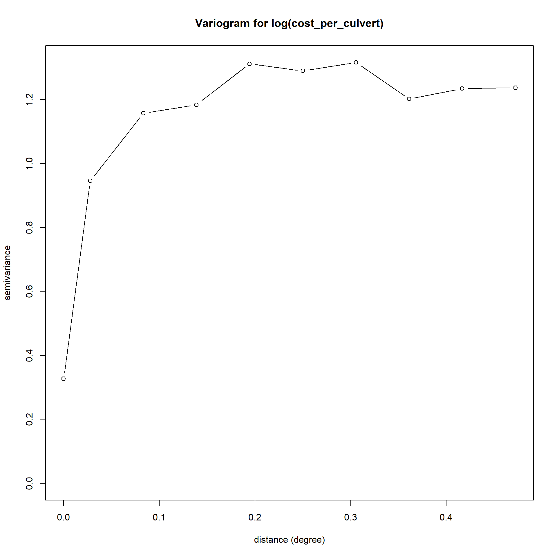
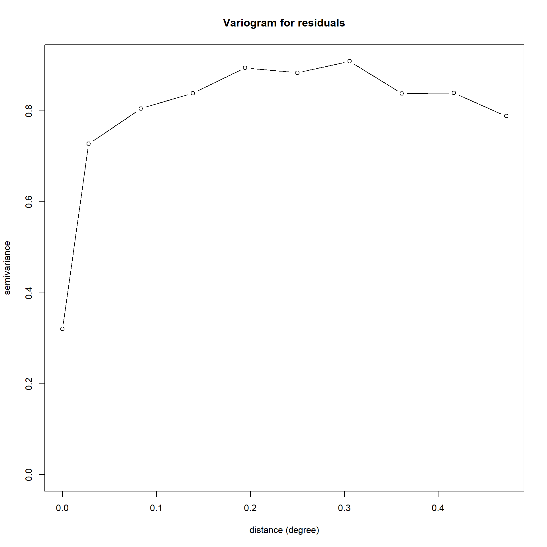
These plots imply that most of the semivariance in both the dependent variable and the error term is captured within a 0.2 degree (or ~20km). We will use this as our threshold for defining which points are neighbors. We also remove 29 worksites with no neighbors (i.e. with no other worksites within 20km) to ensure suitable spatial weighting matrix structure.
Statistical tests of spatial dependence
We use the 20km range established using the above variograms to construct four spatial weighting matrices:
- Distance band specification (Band): weighting matrix is zeros and ones, where wij = wji = 1 when worksite_i is within 20km of worksite_j (assumes all neighbors within buffer have equal dependence).
- Inverse distance decay specification (Decay): weighting matrix is wij = wji = 1/dij where dij is the distance between worksitei and worksitej (assumes dependence decays with distance).
- Hybrid specification (Hybrid): weights are inverse distances when worksite pair is within buffer, and zero otherwise.
- Inverse distance decay with time specification (Decay_t): weights are as the inverse distance decay specification but distances are only computed between worksties that share the same project year. This essentially imposes a restriction of no between-year spatial effects.
For each of these sptail weights specifications, we perform a suite of tests of spatial dependence.
- Moran’s I tests: these tests, performed on both the dependent variable (MoranDep) and the residuals from the model (MoranResid), identify spatial dependence, where the null is no spatial dependence (i.e., distribution over space as good as random).
- Anselin’s Lagrange multiplier tests: these tests of linear restrictions identify mispecification due to spatial dependence, distinguishing whether the source is due to missing spatial lags of the dependent variable or missing spatial error structure, or both. Per Anselin’s suggestion, we consider the robust tests only if both simple tests reject the null.
- LM test against error (LMerr): tests against the null of no spatial error.
- LM test against lag (LMlag): tests against the null of no spatial lag structure.
- Robust LM test against error (RLMerr): a version of LMerr robust to the presence of spatial lag.
- Robust LM test against lag (RLMlag): a version of LMlag robust to the presence of spatial error.
- LMtest against Spatial Autoregressive Moving Average (SARMA): tests against the null of neither spatial error nor spatial lag.
- LM test against error (LMerr): tests against the null of no spatial error.
| Test | Band | Decay | Hybrid | Decay_t |
|---|---|---|---|---|
| MoranDep | 21.42 (<0.001) | 17.254 (<0.001) | 20.817 (<0.001) | 22.465 (<0.001) |
| MoranResid | 5.43 (<0.001) | 11.338 (<0.001) | 12.630 (<0.001) | 14.790 (<0.001) |
| LMerr | 12.75 (<0.001) | 116.293 (<0.001) | 131.817 (<0.001) | 186.455 (<0.001) |
| LMlag | 26.04 (<0.001) | 136.115 (<0.001) | 153.010 (<0.001) | 214.453 (<0.001) |
| RLMerr | 2.27 (0.131) | 0.303 (0.582) | 0.106 (0.744) | 0.457 (0.499) |
| RLMlag | 15.56 (<0.001) | 20.125 (<0.001) | 21.300 (<0.001) | 28.455 (<0.001) |
| SARMA | 28.32 (<0.001) | 136.419 (<0.001) | 153.116 (<0.001) | 214.910 (<0.001) |
| P-values in parentheses |
The Moran test results indicate a strong degree of spatial clustering (or “hot spots”) in both the raw dependent variable and the residuals, though the test statistic shrinks considerably in the residual, suggesting the observed explanatory variables control for a portion of this effect.
For all four weighting schemes, the first-stage LM tests are inconclusive, rejecting the null in all cases. For all three specifications, the robust LM tests indicate a spatial lag specification is more appropriate than the spatial error specification. (The SARMA test suggests that spatial dependence of either type is present.)
Spatial econometric models
Here we present three Cliff-Ord type spatial models, one for each spatial weighting scheme. Based on the preceding tests, we estimate these models with both spatial lag (lambda) terms. We estimate these models via a GMM estimator that accounts for heteroskedastic errors of unknown form (Kelejian and Prucha 2010).
Unfortunately, these estimators do not behave well when other distance-based variables, including the distance to the nearest urban area, density of suppliers, and the basin fixed effect. Therefore, these variables are omitted from these specifications.
| Term | OLS | Band | Decay | Hybrid | Decay w/ Time |
|---|---|---|---|---|---|
| Intercept |
9.92*** (0.253) |
5.3*** (0.688) |
3.42*** (0.802) |
6.13*** (0.66) |
5.29*** (0.676) |
| Stream slope |
-3.96** (1.86) |
-2.29 (1.84) |
-2.87 (1.76) |
-2.66 (1.77) |
-2.7 (1.74) |
| Bankfull width |
-0.00454 (0.00624) |
0.00125 (0.00563) |
-0.00555 (0.00571) |
-0.00204 (0.00551) |
-0.00203 (0.00554) |
| Stream slope X bankfull width |
0.95*** (0.364) |
0.841** (0.387) |
0.75** (0.359) |
0.752** (0.363) |
0.672* (0.343) |
| Road paved (dummy) |
0.198* (0.115) |
0.0773 (0.118) |
0.091 (0.108) |
0.0815 (0.111) |
0.165 (0.106) |
| Road speed class: 3 |
0.635** (0.258) |
0.817** (0.321) |
0.554* (0.311) |
0.627** (0.296) |
0.445 (0.282) |
| Road speed class: 4 |
0.487* (0.26) |
0.538** (0.261) |
0.407* (0.228) |
0.389* (0.236) |
0.29 (0.228) |
| Road speed class: 5 |
0.373*** (0.126) |
0.445*** (0.131) |
0.347*** (0.122) |
0.362*** (0.123) |
0.282** (0.12) |
| Road speed class: 6 |
0.226* (0.137) |
0.333** (0.13) |
0.327*** (0.126) |
0.315** (0.126) |
0.235* (0.122) |
| Road speed class: 7 |
0.25*** (0.0866) |
0.26*** (0.0858) |
0.246*** (0.0782) |
0.219*** (0.0792) |
0.218*** (0.0746) |
| Terrain slope |
0.00735** (0.00354) |
0.000563 (0.00317) |
0.00245 (0.0029) |
0.00257 (0.00289) |
0.00413 (0.00275) |
| Elevation |
-0.000055 (0.000198) |
-0.000369** (0.000155) |
-0.000213* (0.000119) |
-0.000217* (0.000122) |
-0.000185* (0.000112) |
| Land cover: Developed |
0.313*** (0.0759) |
0.244*** (0.0714) |
0.231*** (0.0649) |
0.23*** (0.0665) |
0.222*** (0.0631) |
| Land cover: Herbaceous |
-0.112 (0.176) |
-0.105 (0.112) |
-0.148 (0.108) |
-0.0929 (0.108) |
-0.146 (0.1) |
| Land cover: Planted-cultivated |
0.345** (0.159) |
0.274* (0.143) |
0.281** (0.131) |
0.261* (0.133) |
0.246* (0.135) |
| Land cover: Shrubland |
0.188 (0.13) |
0.241* (0.136) |
0.133 (0.125) |
0.176 (0.125) |
0.142 (0.122) |
| Land cover: Wetlands |
0.072 (0.136) |
0.00935 (0.13) |
0.0422 (0.123) |
0.00513 (0.121) |
0.0196 (0.114) |
| Housing density |
0.000308 (0.00125) |
0.0000732 (0.0017) |
-0.000696 (0.00143) |
-0.00029 (0.00158) |
0.000844 (0.00159) |
| Ag/forestry employment |
0.000148* (0.0000823) |
-0.0000395 (0.0000648) |
-0.0000399 (0.0000604) |
-0.00000691 (0.0000604) |
0.000005 (0.0000578) |
| Construction employment |
-0.0000082 (0.00000925) |
0.00000594 (0.00000708) |
0.00000703 (0.0000069) |
0.00000594 (0.00000672) |
0.00000721 (0.00000661) |
| Private land, individual or company (% 500m buffer) |
-0.00741 (0.105) |
-0.129 (0.102) |
-0.0512 (0.0882) |
-0.0585 (0.0916) |
-0.00956 (0.0862) |
| Private land, managed by industry (% 500m buffer) |
-0.463*** (0.125) |
-0.358*** (0.113) |
-0.33*** (0.104) |
-0.289*** (0.107) |
-0.283*** (0.0976) |
| Private land, managed by non-industrial owner (% 500m buffer) |
0.649*** (0.228) |
0.41* (0.23) |
0.528** (0.232) |
0.458** (0.231) |
0.376* (0.214) |
| Number of worksites |
-0.423*** (0.0574) |
-0.392*** (0.0574) |
-0.327*** (0.0503) |
-0.348*** (0.0518) |
-0.287*** (0.051) |
| Number of worksites X distance |
0.0000484*** (0.0000137) |
0.0000433*** (0.0000136) |
0.0000459*** (0.0000124) |
0.0000449*** (0.0000121) |
0.0000404*** (0.0000107) |
| Culvert installation (dummy) |
0.234* (0.137) |
0.137 (0.106) |
0.217** (0.0997) |
0.16* (0.0969) |
0.286*** (0.09) |
| Culvert removal (dummy) |
0.0262 (0.0821) |
0.0482 (0.0914) |
0.0893 (0.0859) |
0.0673 (0.0856) |
0.123 (0.0787) |
| Project source: BLM |
0.895*** (0.125) |
0.633*** (0.115) |
0.442*** (0.0974) |
0.555*** (0.103) |
0.503*** (0.0997) |
| Project source: HABITAT WORK SCHEDULE |
1.28*** (0.303) |
0.929*** (0.218) |
1.02*** (0.194) |
1.01*** (0.213) |
0.939*** (0.179) |
| Project source: REO |
0.903*** (0.103) |
0.7*** (0.0958) |
0.59*** (0.0892) |
0.646*** (0.0919) |
0.595*** (0.0882) |
| Project source: SRFBD |
1.04*** (0.269) |
0.976*** (0.195) |
1.05*** (0.201) |
1.04*** (0.202) |
0.887*** (0.163) |
| Project source: WA RCO |
0.409* (0.231) |
0.273* (0.165) |
0.561*** (0.142) |
0.394** (0.159) |
0.484*** (0.134) |
| Year: 2002 |
0.196* (0.119) |
0.199* (0.116) |
0.238** (0.11) |
0.194* (0.109) |
‒ |
| Year: 2003 |
0.23* (0.125) |
0.267** (0.125) |
0.237** (0.111) |
0.223** (0.113) |
‒ |
| Year: 2004 |
0.646*** (0.123) |
0.637*** (0.111) |
0.6*** (0.108) |
0.553*** (0.109) |
‒ |
| Year: 2005 |
0.312** (0.124) |
0.314** (0.122) |
0.245** (0.116) |
0.258** (0.116) |
‒ |
| Year: 2006 |
0.386*** (0.131) |
0.324** (0.137) |
0.278** (0.129) |
0.265** (0.129) |
‒ |
| Year: 2007 |
0.54*** (0.141) |
0.624*** (0.14) |
0.498*** (0.135) |
0.48*** (0.135) |
‒ |
| Year: 2008 |
0.0505 (0.225) |
0.193 (0.254) |
0.058 (0.259) |
0.0874 (0.248) |
‒ |
| Year: 2009 |
0.5** (0.204) |
0.358* (0.206) |
0.237 (0.155) |
0.244 (0.163) |
‒ |
| Year: 2010 |
0.149 (0.214) |
0.0685 (0.228) |
0.0992 (0.217) |
-0.00792 (0.223) |
‒ |
| Year: 2011 |
0.201 (0.206) |
0.194 (0.198) |
0.259 (0.19) |
0.2 (0.192) |
‒ |
| Year: 2012 |
-0.138 (0.229) |
-0.127 (0.249) |
-0.0529 (0.231) |
-0.103 (0.216) |
‒ |
| Year: 2013 |
0.0383 (0.201) |
0.0884 (0.243) |
0.0678 (0.258) |
0.0442 (0.249) |
‒ |
| Year: 2014 |
0.16 (0.244) |
0.276 (0.212) |
0.181 (0.221) |
0.173 (0.215) |
‒ |
| Year: 2015 |
0.839* (0.433) |
0.746*** (0.263) |
0.803*** (0.271) |
0.696** (0.288) |
‒ |
| Lambda (lag parameter) | ‒ |
0.472*** (0.0669) |
0.64*** (0.0755) |
0.387*** (0.0645) |
0.477*** (0.0628) |
| * p < 0.1, ** p < 0.05, *** p < 0.01 |
Overall, the conclusions we draw about the associations between costs and the explanatory variables are quite consistent when compared to the basic OLS estimates.
The spatial dependence parameters on all models are positive and statistically significant, indicating positive spatial spillovers from nearby projects. The positive lambdas indicate that more expensive worksites in one location drive up costs nearby. These spillovers are present both between years and within years, as indicated by the positive lambda estimate when the time-dependent weights are used.
Because the spatial lag parameter is non-zero, we cannot interpret the coefficents as direct marginal effects as we would the OLS coefficients. A change in any of the explanatory variables at one worksite impacts not only the worksite’s costs, but also costs at neighboring worksites, which in turn impact costs at the original site. To account for these feedbacks, we can calculate direct, total, and indirect effects. A variable’s direct effect is the effect (in terms of a cost multiplier) of a single unit increase at one worksite on the costs at that same worksite, averaged over all worksites. A variable’s total effect is the effect of a single unit increase at one worksite on costs across all worksites, averaged over all worksites.
Note that a “unit” change in different variables can be quite dramatic. For example, slope is measured on a unit interval though only really ranges fro 0 to about 0.3, so a unit change would be an unrealistic range to expect within the data. In the future, these effects calculations will be scaled to a standard deviation change rather than unit change where appropriate to aid in interpretation.
These calculations are dependent on the spatial structure of the data, and therefore should be interpreted with the following caveat. The worksite data in PNSHP is not comprehensive for all culvert projects in the region during the time period. Because we cannot identify where projects absent in the database were, we cannot fully model the feedback effects that may occur with missing projects in the data. Therefore, I believe these effect calculations will be of limited use.
| Term | Band | Decay | Hybrid | Decay w/ Time |
|---|---|---|---|---|
| Stream slope | 0.0952 / 0.138 / 0.0131 | 0.0374 / 0.00922 / 0.000345 | 0.0595 / 0.221 / 0.0132 | 0.0521 / 0.11 / 0.00571 |
| Bankfull width | 1 / 1 / 1 | 0.994 / 0.991 / 0.985 | 0.998 / 0.999 / 0.997 | 0.998 / 0.998 / 0.996 |
| Stream slope X bankfull width | 2.37 / 2.07 / 4.91 | 2.36 / 3.41 / 8.04 | 2.22 / 1.53 / 3.41 | 2.08 / 1.73 / 3.61 |
| Road paved (dummy) | 1.08 / 1.07 / 1.16 | 1.11 / 1.16 / 1.29 | 1.09 / 1.05 / 1.14 | 1.2 / 1.14 / 1.37 |
| Road speed class: 3 | 2.31 / 2.03 / 4.69 | 1.89 / 2.47 / 4.66 | 1.95 / 1.43 / 2.78 | 1.63 / 1.44 / 2.34 |
| Road speed class: 4 | 1.74 / 1.59 / 2.77 | 1.59 / 1.94 / 3.1 | 1.51 / 1.25 / 1.89 | 1.37 / 1.27 / 1.74 |
| Road speed class: 5 | 1.58 / 1.47 / 2.32 | 1.49 / 1.76 / 2.63 | 1.47 / 1.23 / 1.81 | 1.36 / 1.26 / 1.72 |
| Road speed class: 6 | 1.41 / 1.33 / 1.88 | 1.45 / 1.71 / 2.48 | 1.4 / 1.2 / 1.67 | 1.29 / 1.21 / 1.57 |
| Road speed class: 7 | 1.31 / 1.25 / 1.64 | 1.33 / 1.5 / 1.98 | 1.26 / 1.13 / 1.43 | 1.27 / 1.2 / 1.52 |
| Terrain slope | 1 / 1 / 1 | 1 / 1 / 1.01 | 1 / 1 / 1 | 1 / 1 / 1.01 |
| Elevation | 1 / 1 / 0.999 | 1 / 1 / 0.999 | 1 / 1 / 1 | 1 / 1 / 1 |
| Land cover: Developed | 1.29 / 1.23 / 1.59 | 1.3 / 1.46 / 1.9 | 1.28 / 1.14 / 1.46 | 1.27 / 1.2 / 1.53 |
| Land cover: Herbaceous | 0.898 / 0.913 / 0.82 | 0.844 / 0.785 / 0.662 | 0.906 / 0.949 / 0.859 | 0.852 / 0.887 / 0.756 |
| Land cover: Planted-cultivated | 1.33 / 1.27 / 1.68 | 1.38 / 1.58 / 2.19 | 1.32 / 1.16 / 1.53 | 1.31 / 1.22 / 1.6 |
| Land cover: Shrubland | 1.28 / 1.23 / 1.58 | 1.16 / 1.24 / 1.45 | 1.21 / 1.1 / 1.33 | 1.17 / 1.12 / 1.31 |
| Land cover: Wetlands | 1.01 / 1.01 / 1.02 | 1.05 / 1.07 / 1.12 | 1.01 / 1 / 1.01 | 1.02 / 1.02 / 1.04 |
| Housing density | 1 / 1 / 1 | 0.999 / 0.999 / 0.998 | 1 / 1 / 1 | 1 / 1 / 1 |
| Ag/forestry employment | 1 / 1 / 1 | 1 / 1 / 1 | 1 / 1 / 1 | 1 / 1 / 1 |
| Construction employment | 1 / 1 / 1 | 1 / 1 / 1 | 1 / 1 / 1 | 1 / 1 / 1 |
| Private land, individual or company (% 500m buffer) | 0.875 / 0.894 / 0.783 | 0.943 / 0.92 / 0.867 | 0.94 / 0.967 / 0.909 | 0.99 / 0.992 / 0.982 |
| Private land, managed by industry (% 500m buffer) | 0.692 / 0.734 / 0.508 | 0.685 / 0.583 / 0.399 | 0.736 / 0.849 / 0.624 | 0.734 / 0.794 / 0.583 |
| Private land, managed by non-industrial owner (% 500m buffer) | 1.52 / 1.43 / 2.17 | 1.83 / 2.37 / 4.33 | 1.63 / 1.3 / 2.11 | 1.51 / 1.36 / 2.05 |
| Number of worksites | 0.669 / 0.713 / 0.477 | 0.688 / 0.586 / 0.403 | 0.691 / 0.821 / 0.567 | 0.73 / 0.791 / 0.578 |
| Number of worksites X distance | 1 / 1 / 1 | 1 / 1 / 1 | 1 / 1 / 1 | 1 / 1 / 1 |
| Culvert installation (dummy) | 1.15 / 1.13 / 1.29 | 1.28 / 1.43 / 1.83 | 1.19 / 1.1 / 1.3 | 1.37 / 1.26 / 1.73 |
| Culvert removal (dummy) | 1.05 / 1.04 / 1.1 | 1.11 / 1.16 / 1.28 | 1.07 / 1.04 / 1.12 | 1.14 / 1.11 / 1.27 |
Closing Thoughts
Overall, the spatial econometric methods have little effect on inference regarding the explanatory variables. However, their inclusion does account for an additional source of unobserved variance in the OLS models, while the specific GMM methodology provides robustness against heteroskedastic errors. The spatial parameters themselves provide additional richness to the interpretation of the model. However, given the sparseness of our data, I believe these models are of limited use. Interpreting feedback effects seems particularly challenging, and prediction methods for out-of-sample points are still not particularly well developed. (Definitely no off-the-shelf tools.)
sessionInfo()R version 4.0.2 (2020-06-22)
Platform: x86_64-w64-mingw32/x64 (64-bit)
Running under: Windows 10 x64 (build 19041)
Matrix products: default
locale:
[1] LC_COLLATE=English_United States.1252
[2] LC_CTYPE=English_United States.1252
[3] LC_MONETARY=English_United States.1252
[4] LC_NUMERIC=C
[5] LC_TIME=English_United States.1252
attached base packages:
[1] grid stats graphics grDevices utils datasets methods
[8] base
other attached packages:
[1] lmtest_0.9-37 zoo_1.8-8 sandwich_2.5-1 spatialreg_1.1-7
[5] Matrix_1.2-18 spdep_1.1-5 sf_0.9-5 spData_0.3.8
[9] sp_1.4-4 sphet_1.7-6 fields_11.4 spam_2.5-1
[13] dotCall64_1.0-0 geoR_1.8-1 readxl_1.3.1 ggeffects_1.0.1
[17] margins_0.3.23 broom_0.7.0 kableExtra_1.1.0 knitr_1.29
[21] scales_1.1.1 here_0.1 janitor_2.0.1 forcats_0.5.0
[25] stringr_1.4.0 dplyr_1.0.1 purrr_0.3.4 readr_1.3.1
[29] tidyr_1.1.1 tibble_3.0.4 ggplot2_3.3.2 tidyverse_1.3.0
[33] workflowr_1.6.2
loaded via a namespace (and not attached):
[1] colorspace_1.4-1 deldir_0.1-28 ellipsis_0.3.1
[4] class_7.3-17 sjlabelled_1.1.6 rprojroot_1.3-2
[7] snakecase_0.11.0 fs_1.4.2 rstudioapi_0.11
[10] fansi_0.4.1 lubridate_1.7.9 xml2_1.3.2
[13] codetools_0.2-16 splines_4.0.2 jsonlite_1.7.1
[16] dbplyr_1.4.4 compiler_4.0.2 httr_1.4.2
[19] backports_1.1.8 assertthat_0.2.1 cli_2.1.0
[22] later_1.1.0.1 htmltools_0.5.0 tools_4.0.2
[25] coda_0.19-4 gtable_0.3.0 glue_1.4.2
[28] maps_3.3.0 gmodels_2.18.1 Rcpp_1.0.5
[31] cellranger_1.1.0 raster_3.3-13 vctrs_0.3.4
[34] gdata_2.18.0 nlme_3.1-148 insight_0.12.0
[37] xfun_0.16 ps_1.3.3 rvest_0.3.6
[40] lifecycle_0.2.0 gtools_3.8.2 LearnBayes_2.15.1
[43] MASS_7.3-51.6 hms_0.5.3 promises_1.1.1
[46] expm_0.999-5 yaml_2.2.1 stringi_1.4.6
[49] highr_0.8 e1071_1.7-3 RandomFieldsUtils_0.5.3
[52] boot_1.3-25 rlang_0.4.8 pkgconfig_2.0.3
[55] evaluate_0.14 lattice_0.20-41 prediction_0.3.14
[58] tidyselect_1.1.0 magrittr_1.5 R6_2.4.1
[61] generics_0.0.2 DBI_1.1.0 pillar_1.4.6
[64] haven_2.3.1 withr_2.2.0 units_0.6-7
[67] modelr_0.1.8 crayon_1.3.4 utf8_1.1.4
[70] KernSmooth_2.23-17 rmarkdown_2.3 RandomFields_3.3.8
[73] data.table_1.13.0 blob_1.2.1 git2r_0.27.1
[76] splancs_2.01-40 reprex_0.3.0 digest_0.6.25
[79] classInt_0.4-3 webshot_0.5.2 httpuv_1.5.4
[82] munsell_0.5.0 viridisLite_0.3.0 tcltk_4.0.2