Culvert Cost Machine Learning Methods
B. Van Deynze
March 15, 2021
The goal of these exercises is to explore machine learning methods to improve out-of-sample prediction of culvert improvement costs over predictions from OLS estimates of log-linear average cost models. We loosely follow the methods presented in Hands-On Machine Learning in R by Bradley Boehmke and Brandon Greenwell (available here).
In this process, we split the culvert project cost data randomly into a training and testing set. We then “train” models on the training set, including OLS estimates for comparison. We then “test” these models by computing and comparing Root Mean Square Error (RMSE) of the out-of-sample predictions of the test set.
We consider three related machine learning methods. First, we generate a single regression tree, a method that partitions the data into groups with similar response values (i.e. log average costs) based on discrete splits in the explanatory variables (i.e. land cover is developed or bankfull width is greater than three meters). This partitioning process continues until a stopping point is reached, based either on some penalization per additional “branch” or a set number of splits. Predictions are made by assigning the median value within each group to all members of that group. We compare RMSE across a number of limits to the number of branches, a process known as “pruning.”
We then consider a “bagging” technique known as a random forest (RF), a model-averaging procedure based on bootstrapping (“bagging” is short for “bootstrap aggregating”). This method works by repeatedly randomly selecting a subsample of the training set along with a random selectinon of the potential explanatory varaibles and fitting regression trees for each subsample-variables pair. The final prediction is the mean prediction for each component tree, hence “random forest.”
Finally, we consider the boosted regression tree (BRT) method. This method works through sequential training. A single regression tree is fit to the data, and then a second regression tree is fit to the residuals of the first tree. The predictions from these two models are added together to form an ensemble model, and the residuals from that model are then subsequently fit for an additional tree, and so on and so forth until a stopping point is reached.
We compare testing RMSE and plots of predicted and actual values for each method (including OLS) to determine the preferred method to use in cost predictions out-of-sample (e.g., on the WDFW culvert inventories).
Then, we examine the variables most important to prediction in both of the preferred ML fits. These “importance” metrics are measured as the sum of squared decreases in RMSE at each “node” a variable is associated with across the component models of each fit. This exercise reveals patterns of important predictors quite similar to the set of explanatory variables selected for the OLS fit.
Note that for all methods other than OLS, we provide as an input a nearly complete list of explanatory variables based on the full suite of potentially relevant variables considered throughout the study. This list is presented below.
Parsed with column specification:
cols(
  label = col_character(),
  description = col_character(),
  ols = col_character()
)| Label | Description | Included in OLS? |
|---|---|---|
| basin | Basin (HUC6) containing worksite | X |
| project_source | Organization reporting project to PNSHP | X |
| ua_dist | Distance to Census desginated “urban area” | X |
| uc_dist | Distance to Census designated “urban cluster” | |
| emp_agforest | Number of employees in agriculture and forestry sector in county (Census County Business Patterns data) | X |
| emp_const | Number of employees in construction sector in county (Census County Business Patterns data) | X |
| emp_manuf | Number of employees in manufacturing sector in county (Census County Business Patterns data) | |
| emp_wholesale | Number of employees in wholesale sector in county (Census County Business Patterns data) | |
| emp_retail | Number of employees in retail sector in county (Census County Business Patterns data) | |
| emp_transport | Number of employees in transport sector in county (Census County Business Patterns data) | |
| emp_info | Number of employees in information sector in county (Census County Business Patterns data) | |
| emp_finance | Number of employees in finance sector in county (Census County Business Patterns data) | |
| emp_realestate | Number of employees in real estate sector in county (Census County Business Patterns data) | |
| emp_profsci | Number of employees in professional and science sector in county (Census County Business Patterns data) | |
| emp_admin | Number of employees in administrative sector in county (Census County Business Patterns data) | |
| emp_health | Number of employees in health sector in county (Census County Business Patterns data) | |
| emp_arts | Number of employees in arts sector in county (Census County Business Patterns data) | |
| emp_food | Number of employees in food service sector in county (Census County Business Patterns data) | |
| emp_other | Number of employees in other sectors in county (Census County Business Patterns data) | |
| popdens_cat | Population density in catchement (NHDPlus V2.1 Selected Attributes data) | |
| popdens_acc | … flow accumulated upstream catchements | |
| popdens_tot | … all upstream catchements | |
| hdens_cat | Housing density in catchement (NHDPlus V2.1 Selected Attributes data) | X |
| hdens_acc | … flow accumulated upstream catchements | |
| hdens_tot | … all upstream catchements | |
| nlcd_barren_cat | NLCD barren land cover in catchement (NHDPlus V2.1 Selected Attributes data) | |
| nlcd_barren_acc | … flow accumulated upstream catchements | |
| nlcd_barren_tot | … all upstream catchements | |
| nlcd_crop_cat | NLCD cropland land cover in catchement (NHDPlus V2.1 Selected Attributes data) | |
| nlcd_crop_acc | … flow accumulated upstream catchements | |
| nlcd_crop_tot | … all upstream catchements | |
| nlcd_devhigh_cat | NLCD developed, high-intensity land cover in catchement (NHDPlus V2.1 Selected Attributes data) | |
| nlcd_devhigh_acc | … flow accumulated upstream catchements | |
| nlcd_devhigh_tot | … all upstream catchements | |
| nlcd_devlow_cat | NLCD developed, low-intensity land cover in catchement (NHDPlus V2.1 Selected Attributes data) | |
| nlcd_devlow_acc | … flow accumulated upstream catchements | |
| nlcd_devlow_tot | … all upstream catchements | |
| nlcd_devmed_cat | NLCD developed, medium-intensity land cover in catchement (NHDPlus V2.1 Selected Attributes data) | |
| nlcd_devmed_acc | … flow accumulated upstream catchements | |
| nlcd_devmed_tot | … all upstream catchements | |
| nlcd_devopen_cat | NLCD developed, open space land cover in catchement (NHDPlus V2.1 Selected Attributes data) | |
| nlcd_devopen_acc | … flow accumulated upstream catchements | |
| nlcd_devopen_tot | … all upstream catchements | |
| nlcd_forcon_cat | NLCD forest, coniferous land cover in catchement (NHDPlus V2.1 Selected Attributes data) | |
| nlcd_forcon_acc | … flow accumulated upstream catchements | |
| nlcd_forcon_tot | … all upstream catchements | |
| nlcd_fordec_cat | NLCD forest, deciduous land cover in catchement (NHDPlus V2.1 Selected Attributes data) | |
| nlcd_fordec_acc | … flow accumulated upstream catchements | |
| nlcd_fordec_tot | … all upstream catchements | |
| nlcd_formix_cat | NLCD forest, mixed land cover in catchement (NHDPlus V2.1 Selected Attributes data) | |
| nlcd_formix_acc | … flow accumulated upstream catchements | |
| nlcd_formix_tot | … all upstream catchements | |
| nlcd_grass_cat | NLCD grassland land cover in catchement (NHDPlus V2.1 Selected Attributes data) | |
| nlcd_grass_acc | … flow accumulated upstream catchements | |
| nlcd_grass_tot | … all upstream catchements | |
| nlcd_icesnow_cat | NLCD ice/snow land cover in catchement (NHDPlus V2.1 Selected Attributes data) | |
| nlcd_icesnow_acc | … flow accumulated upstream catchements | |
| nlcd_icesnow_tot | … all upstream catchements | |
| nlcd_nodat_cat | NLCD no data land cover in catchement (NHDPlus V2.1 Selected Attributes data) | |
| nlcd_nodat_acc | … flow accumulated upstream catchements | |
| nlcd_nodat_tot | … all upstream catchements | |
| nlcd_openwater_cat | NLCD open water land cover in catchement (NHDPlus V2.1 Selected Attributes data) | |
| nlcd_openwater_acc | … flow accumulated upstream catchements | |
| nlcd_openwater_tot | … all upstream catchements | |
| nlcd_pasture_cat | NLCD pasture land cover in catchement (NHDPlus V2.1 Selected Attributes data) | |
| nlcd_pasture_acc | … flow accumulated upstream catchements | |
| nlcd_pasture_tot | … all upstream catchements | |
| nlcd_shrub_cat | NLCD shrubland land cover in catchement (NHDPlus V2.1 Selected Attributes data) | |
| nlcd_shrub_acc | … flow accumulated upstream catchements | |
| nlcd_shrub_tot | … all upstream catchements | |
| nlcd_wetherb_cat | NLCD wetland, herbacous land cover in catchement (NHDPlus V2.1 Selected Attributes data) | |
| nlcd_wetherb_acc | … flow accumulated upstream catchements | |
| nlcd_wetherb_tot | … all upstream catchements | |
| nlcd_wetwood_cat | NLCD woody wetland land cover in catchement (NHDPlus V2.1 Selected Attributes data) | |
| nlcd_wetwood_acc | … flow accumulated upstream catchements | |
| nlcd_wetwood_tot | … all upstream catchements | |
| slope | Channel slope (NHDPlus V2.1) | X |
| upst_dist | Upstream routed distance (NHDPlus V2.1) | |
| ppt_cat | Annual precipitation in catchement (NHDPLUS V2.1 Selected Attributes data) | |
| ppt_acc | … flow accumulated upstream catchements | |
| ppt_tot | … all upstream catchements | |
| bfi_cat | Base-flow index in catchement (NHDPLUS V2.1 Selected Attributes data) | |
| bfi_acc | … flow accumulated upstream catchements | |
| bfi_tot | … all upstream catchements | |
| bankfull_width | Bankfull width (NHDPLUS V2.1 Selected Attributes data) | X |
| bankfull_depth | Bankfull depth(NHDPLUS V2.1 Selected Attributes data) | |
| bankfull_xsec_area | Bankfull cross-section area (NHDPLUS V2.1 Selected Attributes data) | |
| cat_streamriver | Proportion of catchement waterways classified as stream/river (NHDPLUS V2.1 Selected Attributes data) | |
| acc_streamriver | … flow accumulated upstream catchements | |
| tot_streamriver | … all upstream catchements | |
| cat_artificial | Proportion of catchement waterways classified as artificial (NHDPLUS V2.1 Selected Attributes data) | |
| acc_artificial | … flow accumulated upstream catchements | |
| tot_artificial | … all upstream catchements | |
| cat_canalditch | Proportion of catchement waterways classified as canal or ditch (NHDPLUS V2.1 Selected Attributes data) | |
| acc_canalditch | … flow accumulated upstream catchements | |
| tot_canalditch | … all upstream catchements | |
| cat_connector | Proportion of catchement waterways classified as connector (NHDPLUS V2.1 Selected Attributes data) | |
| acc_connector | … flow accumulated upstream catchements | |
| tot_connector | … all upstream catchements | |
| cat_pipeline | Proportion of catchement waterways classified as pipeline(NHDPLUS V2.1 Selected Attributes data) | |
| acc_pipeline | … flow accumulated upstream catchements | |
| tot_pipeline | … all upstream catchements | |
| cat_basin_area | Catchement area (NHDPLUS V2.1 Selected Attributes data) | |
| acc_basin_area | … flow accumulated upstream catchements | |
| tot_basin_area | … all upstream catchements | |
| cat_basin_slope | Catchement slope (NHDPLUS V2.1 Selected Attributes data) | X |
| acc_basin_slope | … flow accumulated upstream catchements | |
| tot_basin_slope | … all upstream catchements | |
| cat_elev_mean | Catchement mean elevation (NHDPLUS V2.1 Selected Attributes data) | X |
| acc_elev_mean | … flow accumulated upstream catchements | |
| tot_elev_mean | … all upstream catchements | |
| cat_elev_min | Catchement minimum elevation (NHDPLUS V2.1 Selected Attributes data) | |
| acc_elev_min | … flow accumulated upstream catchements | |
| tot_elev_min | … all upstream catchements | |
| cat_elev_max | Catchement maximum elevation (NHDPLUS V2.1 Selected Attributes data) | |
| acc_elev_max | … flow accumulated upstream catchements | |
| tot_elev_max | … all upstream catchements | |
| cat_stream_slope | Catchement stream slope, mean (NHDPLUS V2.1 Selected Attributes data) | |
| acc_stream_slope | … flow accumulated upstream catchements | |
| tot_stream_slope | … all upstream catchements | |
| cat_stream_length | Catchement main channel length (NHDPLUS V2.1 Selected Attributes data) | |
| acc_stream_length | … flow accumulated upstream catchements | |
| tot_stream_length | … all upstream catchements | |
| cat_rdx | Catchemetn road desnsity (NHDPLUS V2.1 Selected Attributes data) | |
| acc_rdx | … flow accumulated upstream catchements | |
| tot_rdx | … all upstream catchements | |
| sinuosity | Catchement sinuosity, or amount of channel meandering (NHDPLUS V2.1 Selected Attributes data) | |
| cat_strm_dens | Catchement stream density (NHDPLUS V2.1 Selected Attributes data) | |
| acc_strm_dens | … flow accumulated upstream catchements | |
| tot_strm_dens | … all upstream catchements | |
| slope_deg | Slope (°) of GTOPO30 grid cell that culvert restoration site falls within | |
| here_distm | Distance (m) to nearest HERE (formerly NAVTEQ) road within 5000m | |
| here_speed | Speed category of nearest HERE (formerly NAVTEQ) road, worksites over 150m from match assigned to lowest class | X |
| here_class | Functional class of nearest HERE (formerly NAVTEQ) road, worksites over 150m from match assigned to lowest class | |
| here_paved | Is nearest HERE (formerly NAVTEQ) road paved, worksites over 150m from match assigned to lowest class | X |
| here_publi | Is there public access to the nearest HERE (formerly NAVTEQ), worksites over 150m from match assigned to lowest class | |
| hu_type | Type category of 6th field hydrologic unit (“HUC6”) | |
| brick_coun | Kernel density of “Brick, Stone and Related” category based on sites counts | |
| brick_totp | Kernel density of “Brick, Stone and Related” category based on total persons/site | X |
| const_coun | Kernel density of “Construction and Mining” category based on sites counts | |
| const_totp | Kernel density of “Construction and Mining” category based on total persons/site | X |
| merch_coun | Kernel density of all 3 categories (brick…, construction…, metals…) based on sites counts | |
| merch_totp | Kernel density of all 3 categories (brick…, construction…, metals…) based on total persons/site | |
| metal_coun | Kernel density of “Metals Service Centers” category based on sites counts | |
| metal_totp | Kernel density of “Metals Service Centers” category based on total persons/site | X |
| sales_coun | Kernel density of “Sales Yard” category based on sites counts | X |
| sand_count | Kernel density of all categories based on sites counts | |
| bia_5km_buff | Proportion of land owned by the Bureau of Indian Affairs within a 2500m radius of the site | |
| blm_5km_buff | Proportion of land owned by the Bureau of Land Management within a 2500m radius of the site | |
| bpa_5km_buff | Proportion of land owned by the Bonneville Power Administration within a 2500m radius of the site | |
| coe_5km_buff | Proportion of land owned by the Corps of Engineers within a 2500m radius of the site | |
| fws_5km_buff | Proportion of land owned by the U.S. Fish and Wildlife Service within a 2500m radius of the site | |
| gsa_5km_buff | Proportion of land owned by the General Services Administration within a 2500m radius of the site | |
| lg_5km_buff | Proportion of land owned by the Local Government within a 2500m radius of the site | |
| nps_5km_buff | Proportion of land owned by the National Park Service within a 2500m radius of the site | |
| pv_5km_buff | Proportion of land owned by a Private Individual or Company within a 2500m radius of the site | |
| pvi_5km_buff | Proportion of Lands Managed by Private Industry within a 2500m radius of the site | |
| pvn_5km_buff | Proportion of land owned by Private Non-Industrial Owner within a 2500m radius of the site | |
| pvu_5km_buff | Proportion of land owned by Private Urban Lands within a 2500m radius of the site | |
| st_5km_buff | Proportion of land owned by a State Agency within a 2500m radius of the site | |
| stf_5km_buff | Proportion of land owned by the State Dept. of Forestry within a 2500m radius of the site | |
| stl_5km_buff | Proportion of land owned by the Division of State Lands within a 2500m radius of the site | |
| stp_5km_buff | Proportion of land owned by the State Dept. of Parks and Recreation within a 2500m radius of the site | |
| stw_5km_buff | Proportion of land owned by the State Dept. of Fish and Wildlife within a 2500m radius of the site | |
| und_5km_buff | Proportion of land where ownership is Undetermined within a 2500m radius of the site | |
| usfs_5km_buff | Proportion of land owned by the U.S. Forest Service within a 2500m radius of the site | |
| water_5km_buff | Proportion of land that is Water within a 2500m radius of the site | |
| bia_2km_buff | Proportion of land owned by the Bureau of Indian Affairs within a 1000m radius of the site | |
| blm_2km_buff | Proportion of land owned by the Bureau of Land Management within a 1000m radius of the site | |
| bpa_2km_buff | Proportion of land owned by the Bonneville Power Administration within a 1000m radius of the site | |
| coe_2km_buff | Proportion of land owned by the Corps of Engineers within a 1000m radius of the site | |
| fws_2km_buff | Proportion of land owned by the U.S. Fish and Wildlife Service within a 1000m radius of the site | |
| gsa_2km_buff | Proportion of land owned by the General Services Administration within a 1000m radius of the site | |
| lg_2km_buff | Proportion of land owned by the Local Government within a 1000m radius of the site | |
| nps_2km_buff | Proportion of land owned by the National Park Service within a 1000m radius of the site | |
| pv_2km_buff | Proportion of land owned by a Private Individual or Company within a 1000m radius of the site | |
| pvi_2km_buff | Proportion of Lands Managed by Private Industry within a 1000m radius of the site | |
| pvn_2km_buff | Proportion of land owned by Private Non-Industrial Owner within a 1000m radius of the site | |
| pvu_2km_buff | Proportion of land owned by Private Urban Lands within a 1000m radius of the site | |
| st_2km_buff | Proportion of land owned by a State Agency within a 1000m radius of the site | |
| stf_2km_buff | Proportion of land owned by the State Dept. of Forestry within a 1000m radius of the site | |
| stl_2km_buff | Proportion of land owned by the Division of State Lands within a 1000m radius of the site | |
| stp_2km_buff | Proportion of land owned by the State Dept. of Parks and Recreation within a 1000m radius of the site | |
| stw_2km_buff | Proportion of land owned by the State Dept. of Fish and Wildlife within a 1000m radius of the site | |
| und_2km_buff | Proportion of land where ownership is Undetermined within a 1000m radius of the site | |
| usfs_2km_buff | Proportion of land owned by the U.S. Forest Service within a 1000m radius of the site | |
| water_2km_buff | Proportion of land that is Water within a 1000m radius of the site | |
| bia_1km_buff | Proportion of land owned by the Bureau of Indian Affairs within a 500m radius of the site | |
| blm_1km_buff | Proportion of land owned by the Bureau of Land Management within a 500m radius of the site | |
| bpa_1km_buff | Proportion of land owned by the Bonneville Power Administration within a 500m radius of the site | |
| coe_1km_buff | Proportion of land owned by the Corps of Engineers within a 500m radius of the site | |
| fws_1km_buff | Proportion of land owned by the U.S. Fish and Wildlife Service within a 500m radius of the site | |
| gsa_1km_buff | Proportion of land owned by the General Services Administration within a 500m radius of the site | |
| lg_1km_buff | Proportion of land owned by the Local Government within a 500m radius of the site | |
| nps_1km_buff | Proportion of land owned by the National Park Service within a 500m radius of the site | |
| pv_1km_buff | Proportion of land owned by a Private Individual or Company within a 500m radius of the site | X |
| pvi_1km_buff | Proportion of Lands Managed by Private Industry within a 500m radius of the site | X |
| pvn_1km_buff | Proportion of land owned by Private Non-Industrial Owner within a 500m radius of the site | X |
| pvu_1km_buff | Proportion of land owned by Private Urban Lands within a 500m radius of the site | |
| st_1km_buff | Proportion of land owned by a State Agency within a 500m radius of the site | |
| stf_1km_buff | Proportion of land owned by the State Dept. of Forestry within a 500m radius of the site | |
| stl_1km_buff | Proportion of land owned by the Division of State Lands within a 500m radius of the site | |
| stp_1km_buff | Proportion of land owned by the State Dept. of Parks and Recreation within a 500m radius of the site | |
| stw_1km_buff | Proportion of land owned by the State Dept. of Fish and Wildlife within a 500m radius of the site | |
| und_1km_buff | Proportion of land where ownership is Undetermined within a 500m radius of the site | |
| usfs_1km_buff | Proportion of land owned by the U.S. Forest Service within a 500m radius of the site | |
| water_1km_buff | Proportion of land that is Water within a 500m radius of the site | |
| project_year | Year work on project began | X |
| n_worksites | Number of worksites assoicated with project | X |
| n_culverts | Numbr of culverts assocated with worksite | |
| action_fishpass_culvimp_prj | Indicator if project involves any culvert improvement actions | X |
| action_fishpass_culvinst_prj | Indicator if project involves any culvert installation actions | |
| action_fishpass_culvrem_prj | Indicator if project involves any culvert removal actions | X |
| action_fishpass_culvimp_count_prj | Count of culvert improvement actions across project | |
| action_fishpass_culvinst_count_prj | Count of culvert installation actions across project | |
| action_fishpass_culvrem_count_prj | Count of culvert removal actions across project | |
| action_fishpass_culvimp_wrk | Indicator if worksite involves any culvert improvement actions | |
| action_fishpass_culvinst_wrk | Indicator if worksite involves any culvert installation actions | |
| action_fishpass_culvrem_wrk | Indicator if worksite involves any culvert removal actions | |
| action_fishpass_culvimp_count_wrk | Count of culvert improvement actions at worksite | |
| action_fishpass_culvinst_count_wrk | Count of culvert installation actions at worksite | |
| action_fishpass_culvrem_count_wrk | Count of culvert removal actions at worksite | |
| dist_max | Maximum distance between worksites | |
| dist_mean | Mean distance between worksites | |
| here_class_0 | HERE road class with no accuracy check | |
| here_class_badmatch | HERE road class with bad matches assigned own class | |
| here_speed_0 | HERE speed class with no accuracy check | |
| here_speed_badmatch | HERE speed class with bad matches assigned own class | |
| here_paved_0 | HERE paved indicator with no accuracy check | |
| pvall_5km_buff | Sum of all private land classes, 2500m radius buffer | |
| stall_5km_buff | Sum of all state-managed land classes, 2500m radius buffer | |
| fedother_5km_buff | Sum of smaller federally-managed land classes, 2500m radius buffer | |
| pvall_2km_buff | Sum of all private land classes, 1000m radius buffer | |
| stall_2km_buff | Sum of all state-managed land classes, 1000m radius buffer | |
| fedother_2km_buff | Sum of smaller federally-managed land classes, 1000m radius buffer | |
| pvall_1km_buff | Sum of all private land classes, 500m radius buffer | |
| stall_1km_buff | Sum of all state-managed land classes, 500m radius buffer | |
| fedother_1km_buff | Sum of smaller federally-managed land classes, 500m radius buffer | |
| tot_dist | Total distance between worksites | X |
| nlcd_current_class | NLCD land cover at worksite point for project year, aggregated categories | X |
| nlcd_current_fullclass | NLCD land cover at worksite point for project year |
Machine learning methods
Regression tree
We start with a number of simple regression trees. To begin, we randomly assign half the sample to a “training” set which we will use to fit the models.
# Select training group (half the total observations, used to build the model, remaining obs are used as out-of-sample test group)
set.seed(1)
train = sample(1:nrow(df_tree), nrow(df_tree)/2)
Then, we use the rpart package to fit and plot a regression tree using the training data.
# Build a single regression tree
library(rpart)
library(rpart.plot)
set.seed(1)
tree_culv <- rpart(log(cost_per_culvert) ~ ., df_tree, subset = train)
rpart.plot(tree_culv, digits = 3)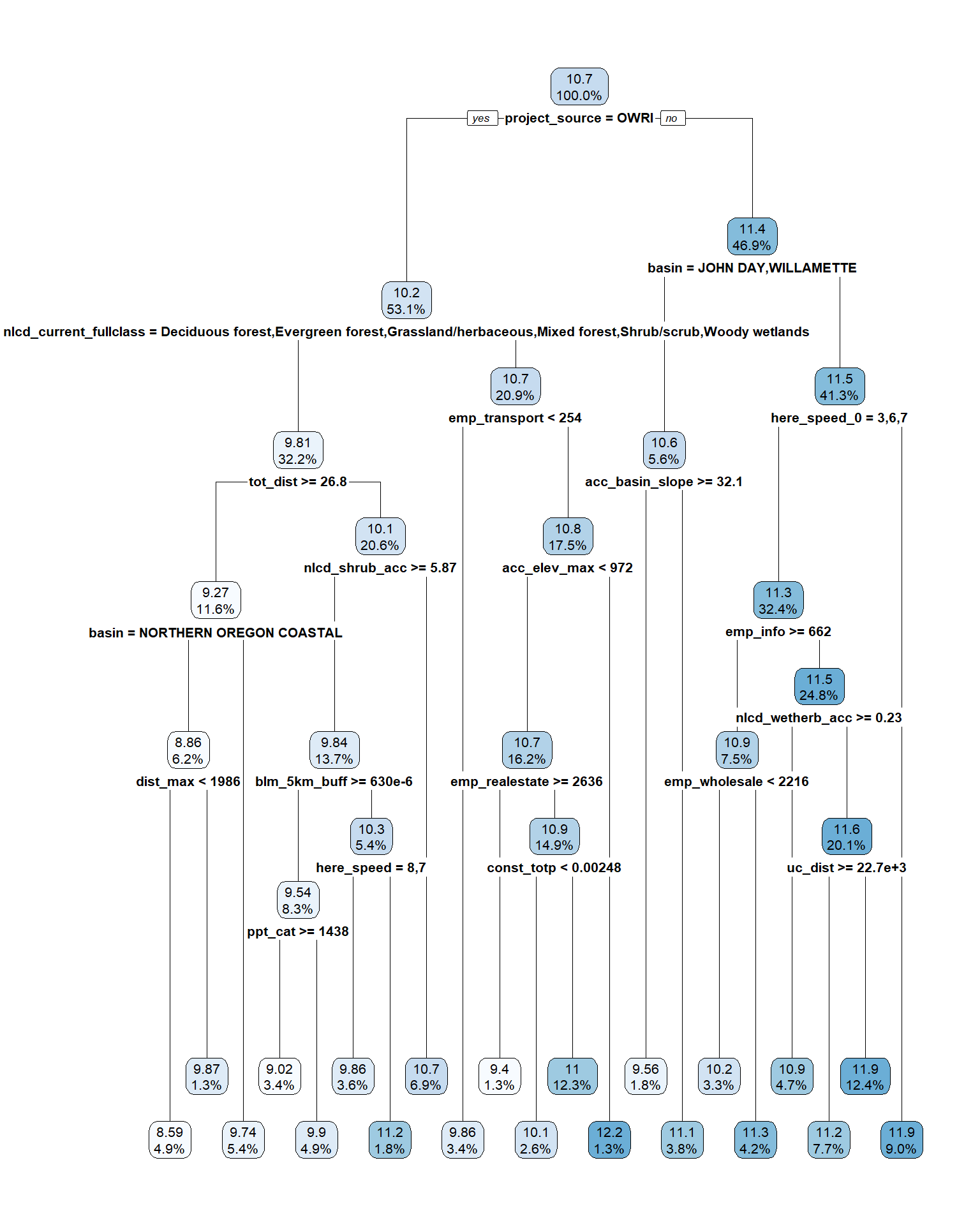
In each “leaf” the number is the median log(cost) of all worksites in the set that passes all the qualifiers above Each “branch” assigns worksites to the left if it passes the qualifier, right otherwise (YES –> left; No –> right), and the percent of the sample assigned to each node. Fixed effects like project source and basin appear important, though which other variables are selected for splits is highly dependent on the specific sample randomly chosen for the training set. That said, some variables such as distance to urban areas, distance between worksites, land cover, land ownership, and employment measures are all represented in ways similar to the OLS results.
Note that the rpart package automatically “prunes” the tree to the “optimal” number of leaves using a 10-fold cross validation, using different complexity cost parameters and comparing the relative error on the testing set and selecting the number of nodes that minimizes that error (or a meaningful improvements are not found my increasing the number of leaves). We can look at the relative error as a function of the complexity cost parameter (cp, which in effect limits the number of leaves).
plotcp(tree_culv)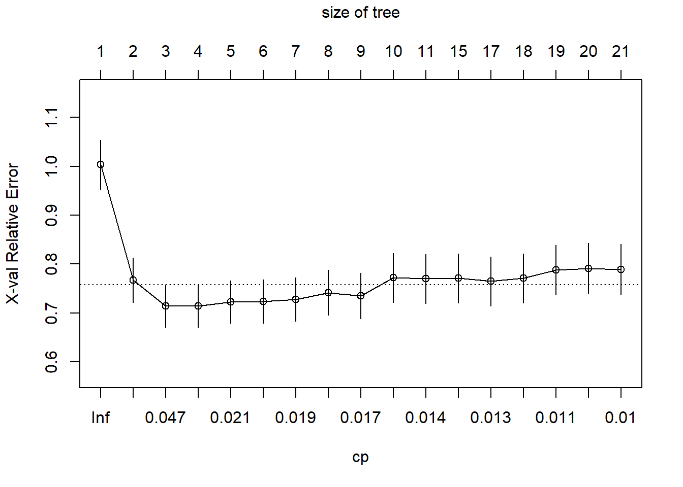
It looks like using the default 21 leaf tree in fact might be over-fitting the model, so we will also look at a smaller four-leaf tree, which looks like it should provide better predictions.
tree_culv_4 <- rpart(log(cost_per_culvert) ~ ., df_tree, subset = train, control = list(cp = 0.025))
rpart.plot(tree_culv_4, digits = 3)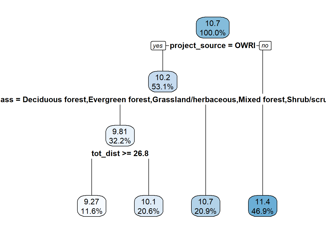
In this smaller tree, reporting source, land cover, and the total distance between worksites are the variables used to split the sample. Note that tot_dist has a counter intuitive effect: worksites further apart from other worksites under the same project are cheaper. Note that this is likely because tot_dist is proxying for the number of worksites here. Projects with only one worksite that do not benefit from scale economies will have tot_dist values of zero, and so this effect is captured by the distance.
One thing to think about is that project year, project source, and the number of worksites are all variables impossible to really observe for true out-of-sample culverts. These variables drive a lot of the cost variation, but the OLS model with fixed effects allows us to make predictions out-of-sample by “averaging” over these effects. We can do this for the trees too, but not sure it will be as useful if these features/variables drive most of the prediction (as is the case with the four leaf tree).
Random forest (RF)
This method uses “bagging”, or bootstrap aggregating, to boostrap sample the training set a fixed number (N) of times (1,000 here) and generate a tree using a fixed number (M) of randomly selected candidate variables. The resulting model averages predictions over all the generated trees in the “forest”.
library(randomForest)
set.seed(1)
bag_culv <- randomForest(log(cost_per_culvert) ~ ., data = df_tree, subset = train, mtry = 25, ntree = 1000, importance = TRUE)
# Looks like a good chance this is better than both the OLS and individual trees
Because these fits aggregate hundreds of trees like those seen in the preceding section, they are vastly less interpretable. We will look at the relative importance of the explanatory variables across the models later in this report.
Boosted regression tree (BRT)
This method is similar to the bagging method above in that it generates a “random forest”. Unlike the random forest above, each underlying “tree” in the “forest” is build sequentially on the residuals of the previous tree, so that each successive tree added results in improved prediction accuracy of the ensemble model (the forest). It proceeds using gradient descent method until it thinks it has found the global minimum for some loss function (here RMSE/SSE/MSE equivalently).
library(gbm)
set.seed(1)

# Takes ~1min to fun on my machine
boost_culv <- gbm(log(cost_per_culvert) ~ ., data = df_tree[train,], distribution = "gaussian", n.trees = 5000, interaction.depth = 4, cv.folds = 5)
Again, these trees are difficult to interpret because they aggregate several component models. Therefore, we will wait to look at relative performance and variable importance until the next section.
Variable importance plots
We present plots of relative variable importance for both RF and BRT methods. Variable importance is defined as the sum of squared improvements (in mean squared error) for every node where a variable is selected. For ensemble models like RF and BRT, these improvements are averaged across all component trees.
grid.arrange(
vip(bag_culv, num_features = 25, geom = "point", aesthetics = list(size = 4, color = scales::brewer_pal("qual", 1)(6)[5])) +
  labs(
    x = NULL, y = "Importance", title = "RF"
  ) +
  theme_bw() +
  theme(
    plot.background = element_rect(color = NULL), legend.position = "none"
  ),
vip(boost_culv, num_features = 25, geom = "point", aesthetics = list(size = 4, color = scales::brewer_pal("qual", 1)(6)[2])) +
  labs(
    x = NULL, y = "Importance", title = "BRT"
  ) +
  theme_bw() +
  theme(
    plot.background = element_rect(color = NULL), legend.position = "none"
  ),
nrow = 1
)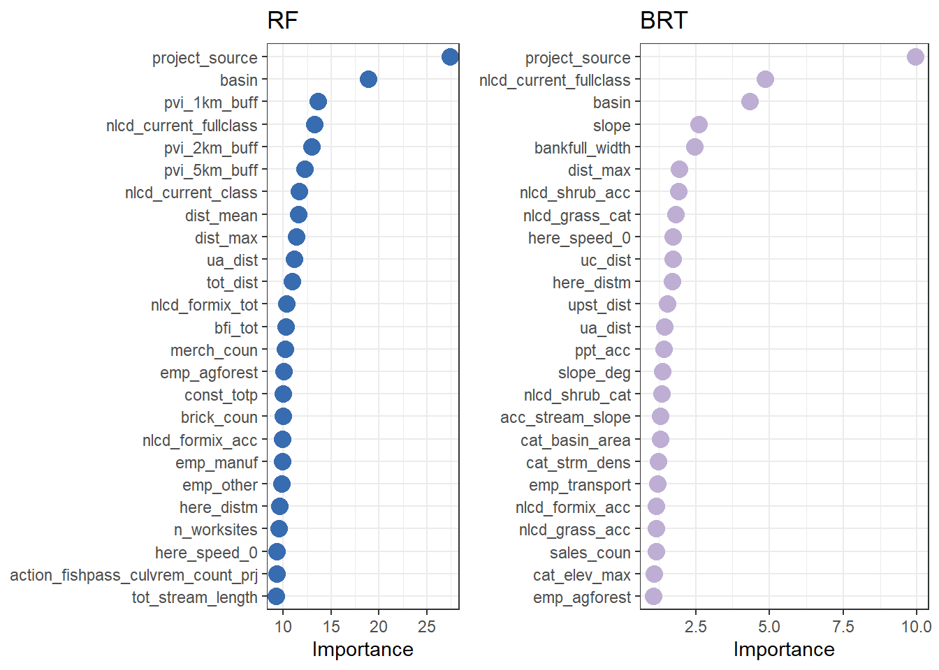
Many of the variables included in the OLS model appear within the top 25 most important variables in one or both of the ML models. In particular, project source and basin explain a huge amount of the variation in the data, consistent with the fixed effects estimates using OLS. NLCD land cover also plays a large role in both fits. Road features (speed class, distance to road line) play important roles in both fits as well, consistent with the OLS estimates.
Private land managed by industry, measured at all distances, is very important in the RF fit. Project scale effects like number of worksites, and maximum, mean, and total distance between worksites also play important roles in the RF fit, as do measures of employment by sector and supplier density. In the BRT, hydrological features play a more important role, with bankfull_width and slope both standing out. On the whole, the variables we select for the OLS fit seem to be similar to the features that play the most important role in prediction.
Relative predictive power
# ____ Compare RMSE ----Root mean square error (RMSE) by method
tibble(
  "OLS" = rmse_ols,
  "4-leaf tree" = rmse_tree4,
  # "rmse_tree10" = rmse_tree10,
  "Full tree" = rmse_treefull,
  "RF" = rmse_bag,
  "BRT" = rmse_boost
) %>%
  pivot_longer(everything(), names_to = "method", values_to = "rmse") %>%
  ggplot(
    aes(
      x = reorder(method, rmse),
      y = rmse,
      fill = method
    )
  ) +
  geom_hline(aes(yintercept = rmse_ols), data = . %>% filter(method == "rmse_ols"), linetype = "dashed") +
  geom_col(aes(fill = method), color = "black") +
  geom_hline(yintercept = 0) +
  geom_text(aes(label = round(rmse, 3), y = rmse + 0.025)) +
  scale_fill_brewer(type = "qual") +
  # scale_color_brewer(type = "qual") +
  labs(
    x = NULL, y = "RMSE", title = "RMSE by method (testing set)",
    subtitle = "RF shows lowest RMSE, followed closely by BRT, representing ~10% and 7% increase in prediction accuracy over OLS respectively"
  ) +
  theme_bw() +
  theme(
    plot.background = element_rect(color = NULL), legend.position = "none"
  )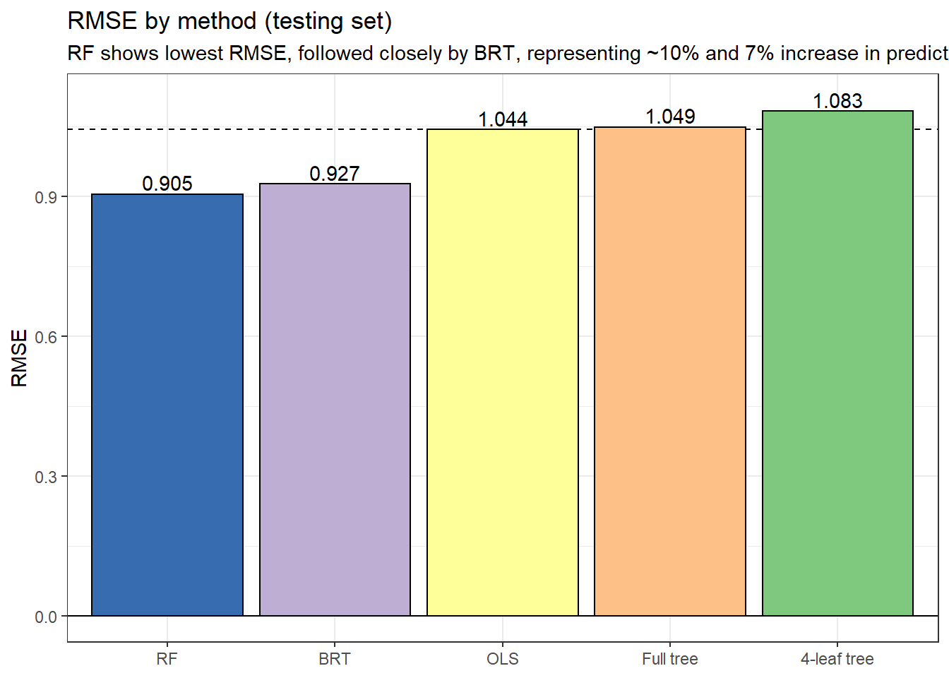
We compare RMSE calculated using the testing set (the subsample withheld during fitting) to compare out-of-sample predictive power. Compared to the OLS baseline, the basic regression trees actually perform somewhat worse, while both of the model aggregation methods (RF and BRT) perform signficantly better.
# ____ Compare fitted vs. observed plots ----Fitted vs. actual plots
df_yhats <-
  tibble(
    "y" = log(df_tree$cost_per_culvert[-train]),
    "OLS" = yhat_culv_ols,
    "4-leaf tree" = yhat_culv_4,
    # "yhat_tree10" = yhat_culv_10,
    "Full tree" = yhat_culv,
    "RF" = yhat_culv_bag,
    "BRT" = yhat_boost
  ) %>%
  pivot_longer(
    -y
  )
df_yhats %>%
  ggplot(
    aes(
      x = y,
      y = value,
      fill = name
    )
  ) +
  geom_abline(slope = 1) +
  geom_point(shape = 21, stroke = 0.4) +
  facet_wrap(~ name) +
  scale_fill_brewer(type = "qual") +
  # scale_color_brewer(type = "qual") +
  labs(
    x = "Actual cost (log-scale)", y = "Predicted cost (log-scale)", title = "Predicted vs. actual costs (testing set)",
    subtitle = "RF demonstrates an unfortunate skew"
  ) +
  theme_bw() +
  theme(
    plot.background = element_rect(color = NULL), legend.position = "none"
  ) +
  scale_x_continuous(labels = function(x) scales::dollar(exp(x)), breaks = c(log(3000), log(22000), log(150000))) +
  scale_y_continuous(labels = function(x) scales::dollar(exp(x)), breaks = c(log(3000), log(22000), log(150000)))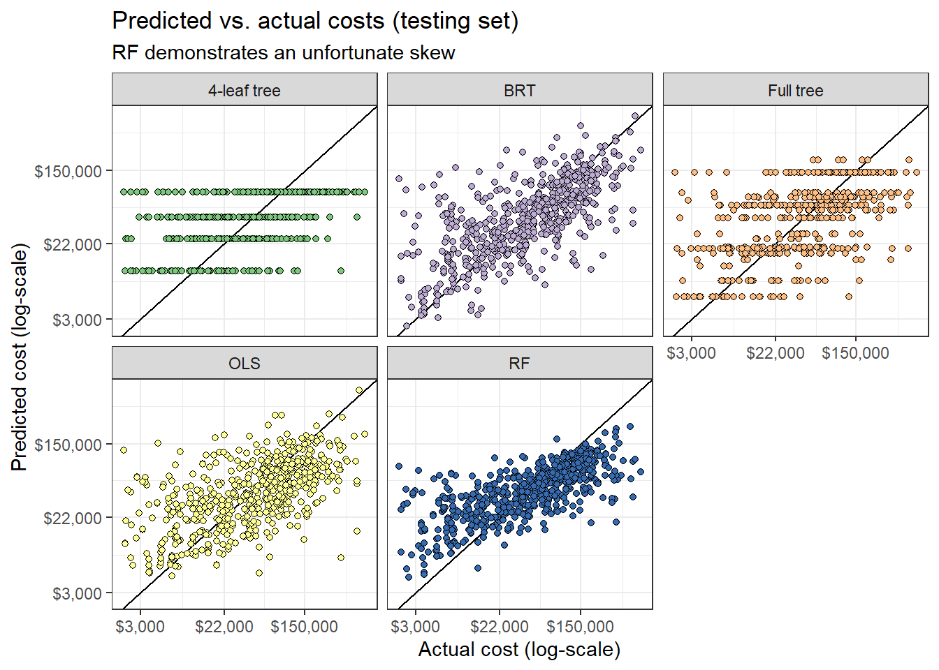
Looking at the predictions against the actual costs per culvert values, we see the limits of the simple regression trees, which places each worksite into one of only a handful of bins. The aggregating methods RF and BRT perform much more similarly to OLS, providing predictions distinct for each worksite. Notice that while RF has a lower RMSE, it tends to over-estimate costs for cheaper projects and under-estimate costs for more expensive ones, which may distort the underlying variability in costs across the landscape.
Redisual distribtuions
df_yhats %>% mutate(resid = y - value) %>%
ggplot(
  aes(
    x = resid,
    # color = name,
    fill = name
  )
) +
  geom_density(alpha = 0.8, color = "black") +
  geom_vline(xintercept = 0, linetype = "dashed") +
  facet_wrap(~ name) +
  scale_fill_brewer(type = "qual") +
  # scale_color_brewer(type = "qual") +
  labs(
    x = "Residual (log-cost)", y = "Density", title = "Residual distribution (testing set)",
    subtitle = "BRT has tighter clustering of residuals near zero but wider tails"
  ) +
  theme_bw() +
  theme(
    plot.background = element_rect(color = NULL), legend.position = "none"
) 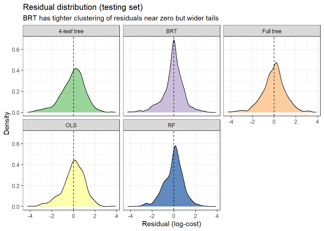
# scale_x_continuous(labels = function(x) comma(exp(x), 0.1), breaks = c(-3, -1.5, 0, 1.5, 3))Here we plot the density of residuals from all five methods. Notice that BRT has a tighter peak near zero compared to even the RF plot. This suggests that though RF provides a lower out-of-sample RMSE, BRT predictions may more consistently hit the mark. However, for BRT to display this sharp peak of near zero-residuals and still have a larger RMSE, it must mean that when it misses, it misses worse, indicated here by longer tails.
Conclusions
The boosted regression tree has several desirable properties as an estimator of conditional cost distributions:
- It provides metrics to compare variable importance and plots of conditional mean costs, allowing comparison to inference from OLS (and spatial regression)
- While its RMSE is a bit higher (~3%) than random forest (bagging), its predictions are much tighter (RMSE growth is driven by longer tails)
Further investigation is warranted to see if we can train specifically for improved performance in specific areas, such as Puget Sound, for the purposes of targeted planning tools.
sessionInfo()R version 4.0.2 (2020-06-22)
Platform: x86_64-w64-mingw32/x64 (64-bit)
Running under: Windows 10 x64 (build 19041)
Matrix products: default
locale:
[1] LC_COLLATE=English_United States.1252
[2] LC_CTYPE=English_United States.1252
[3] LC_MONETARY=English_United States.1252
[4] LC_NUMERIC=C
[5] LC_TIME=English_United States.1252
attached base packages:
[1] stats graphics grDevices utils datasets methods base
other attached packages:
[1] gbm_2.1.8 randomForest_4.6-14 rpart.plot_3.0.9
[4] rpart_4.1-15 MASS_7.3-51.6 kableExtra_1.1.0
[7] knitr_1.29 pdp_0.7.0 vip_0.3.2
[10] lmtest_0.9-37 zoo_1.8-8 sandwich_2.5-1
[13] readxl_1.3.1 here_0.1 janitor_2.0.1
[16] forcats_0.5.0 stringr_1.4.0 dplyr_1.0.1
[19] purrr_0.3.4 readr_1.3.1 tidyr_1.1.1
[22] tibble_3.0.4 ggplot2_3.3.2 tidyverse_1.3.0
[25] searchable_0.3.3.1 workflowr_1.6.2
loaded via a namespace (and not attached):
[1] fs_1.4.2 lubridate_1.7.9 RColorBrewer_1.1-2 webshot_0.5.2
[5] httr_1.4.2 rprojroot_1.3-2 tools_4.0.2 backports_1.1.8
[9] utf8_1.1.4 R6_2.4.1 DBI_1.1.0 colorspace_1.4-1
[13] withr_2.2.0 tidyselect_1.1.0 gridExtra_2.3 compiler_4.0.2
[17] git2r_0.27.1 cli_2.1.0 rvest_0.3.6 xml2_1.3.2
[21] labeling_0.3 scales_1.1.1 digest_0.6.25 rmarkdown_2.3
[25] pkgconfig_2.0.3 htmltools_0.5.0 dbplyr_1.4.4 highr_0.8
[29] rlang_0.4.8 rstudioapi_0.11 farver_2.0.3 generics_0.0.2
[33] jsonlite_1.7.1 magrittr_1.5 Matrix_1.2-18 Rcpp_1.0.5
[37] munsell_0.5.0 fansi_0.4.1 lifecycle_0.2.0 stringi_1.4.6
[41] yaml_2.2.1 snakecase_0.11.0 grid_4.0.2 blob_1.2.1
[45] parallel_4.0.2 promises_1.1.1 crayon_1.3.4 lattice_0.20-41
[49] haven_2.3.1 splines_4.0.2 hms_0.5.3 ps_1.3.3
[53] pillar_1.4.6 reprex_0.3.0 glue_1.4.2 evaluate_0.14
[57] modelr_0.1.8 vctrs_0.3.4 httpuv_1.5.4 cellranger_1.1.0
[61] gtable_0.3.0 assertthat_0.2.1 xfun_0.16 broom_0.7.0
[65] later_1.1.0.1 survival_3.1-12 viridisLite_0.3.0 ellipsis_0.3.1