Summary of Spatially Derived Variables for Culvert Projects
B. Van Deynze
March 15, 2021
This document summarizes spatially-derived variables for PNSHP culvert work sites. These variables are collected by linking the worksite points to other spatial data sets via polygon covers or identifying the nearest line. Variables were selected for their value as either potential drivers of project cost, or as potential proxies for ecological benefits.
As of right now, we have data from Blake on roads, streams, habitat use, slope, and land cover. I also have collected some county-level data on employment levels in relevant sectors. With some help from Sunny, I also pulled the nearest NHD+ stream COMID, which was used to link a number of additional variables related to stream, land cover, and population features of the stream and upstream basins.
In the first section, I summarize data sources and define important variables. In the next section, I evaluate the quality of matches for road and stream data. In the third sections, I present descriptive figures for the new variables. And, finally, I close with some early regression results incorporating the new variables.
Data sources and variable definitions
Culvert worksite data
Data on culvert worksite locations and associated project information (reporting source, project cost, year), are from the Pacific Northwest Salmon Habitat Projects database, which documents projects relevant to salmonid habitat restoration, including culvert improvements. We restrict the sample to projects that:
- Only include culvert actions across any worksites;
- Were completed between 2001 and 2015;
- Were located only in Washington or Oregon;
- Were reported by a source that reports more than 20 total projects;
- Were located in basins with over 20 worksites reported;
- Reported project costs per culvert between $2,000 and $750,000 (roughly 5th and 95th percentiles of all reported project costs).
Evaluating accuracy of stream and road matches
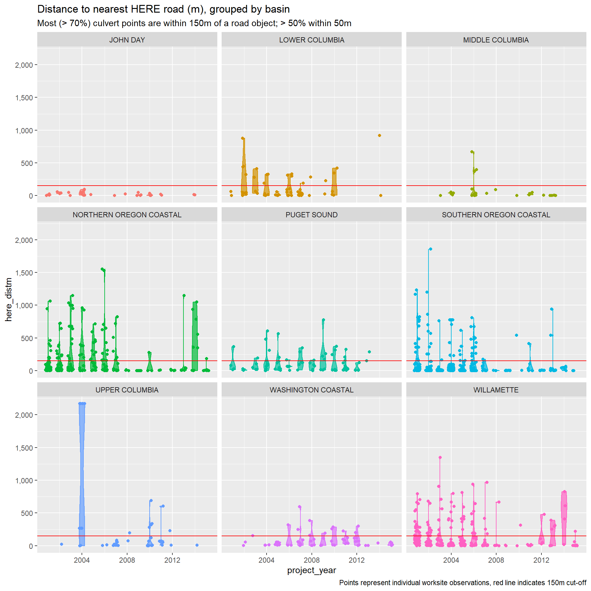
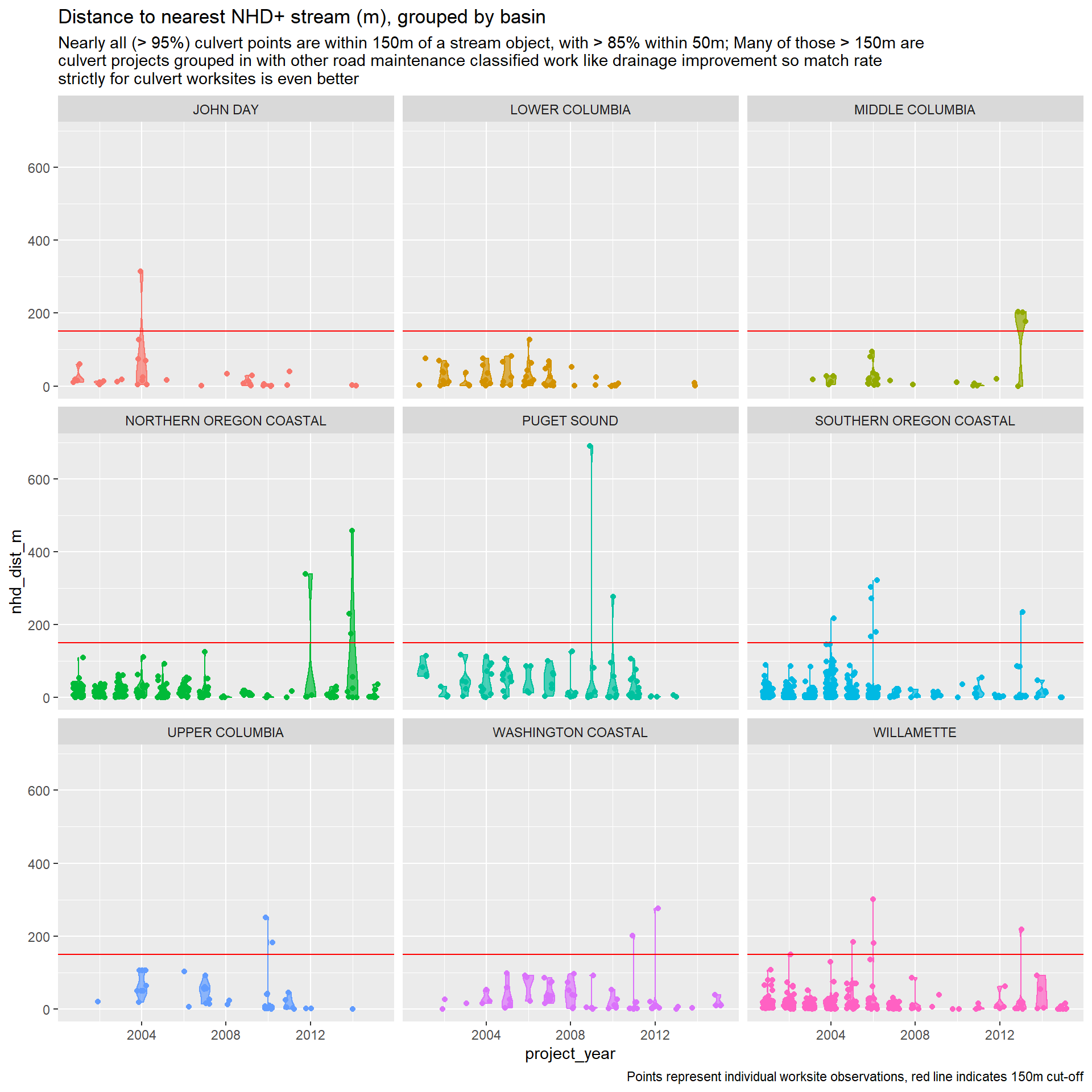
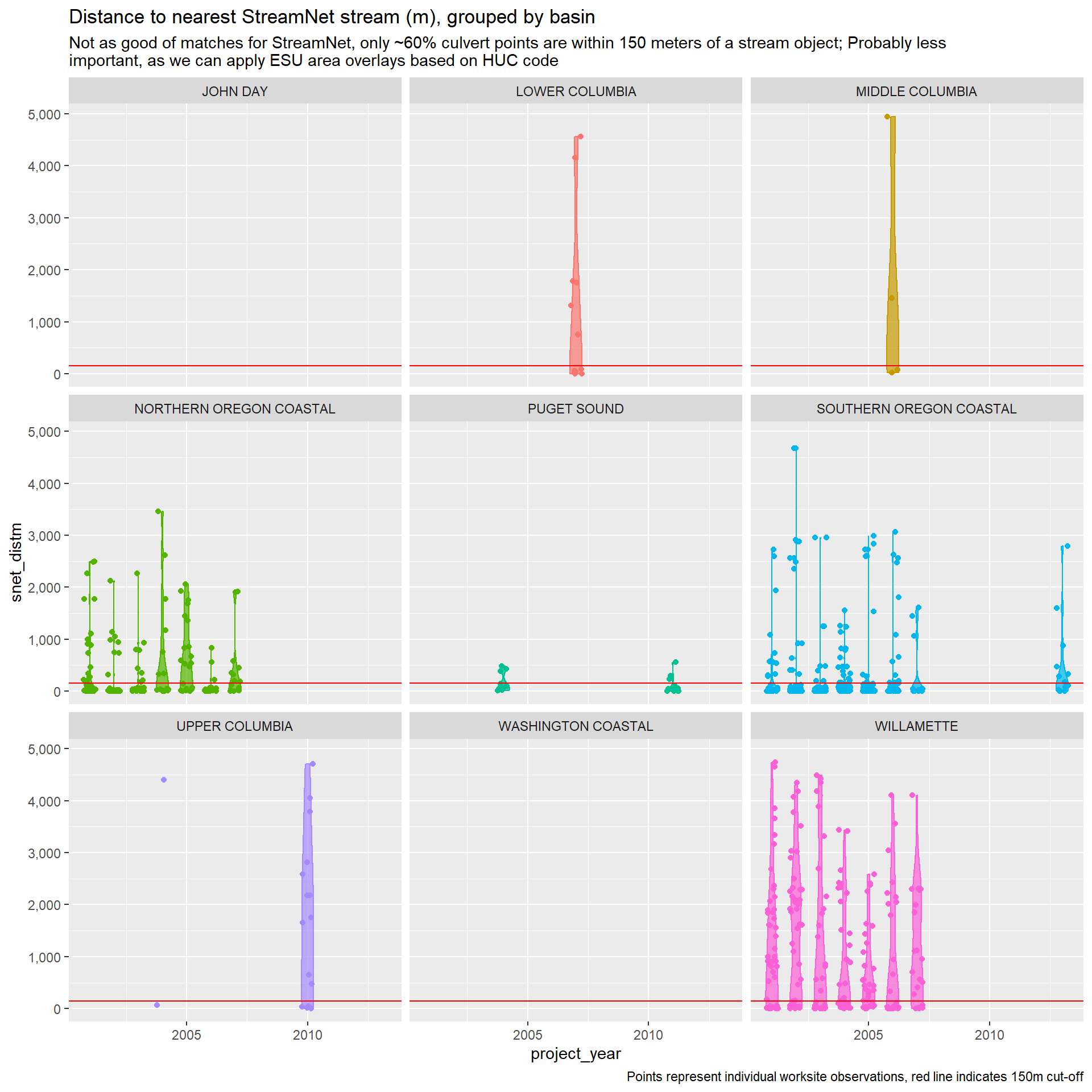
First thing we’ll do is check how accurate the culvert worksite points match up with the road and stream data recovered from three sources: (1) HERE for network-able road features, (2) NHDPlus HR for stream/river classification and features, (3) StreamNet for salmonid habitat use data by species. We will evaluate the precision of matches using distance to the “matching” line, measured in meters.
We suspect two possible sources of imprecision. First, worksite points may be reported with imprecision, in which case the match would represent the most likely feature, but with less certainty than if distance was lower. Second, the worksite may be on a road or stream that is not represented in our source data. In this case, the matched feature would misrepresent the true feature we are trying to identify for the worksite.
In either case, we will need to identify and decide how to deal with “poor” matches. For now, we will define poor matches as worksites over 150m from the target feature (i.e. road or stream), represented in the figures below with a red horizontal line. This threshold is easily adjustable, and sensitivity to this threshold will also be examined.
Dealing with poor matches
So StreamNet’s less dense streams have the worst matches, while NHDPlus has very close matches. StreamNet is most useful for salmon habitat identification, though HUC code based habitat maps can be used instead (e.g. maps seen in Crozier et al. (2018)). I think using this approach might be preferred for consistency, given the large number of poor matches in the StreamNet data. For the cost modeling stage, this variables is less important. For StreamNet, wait for next steps.
The HERE roads have lots of close matches, but also plenty that are far off the mark. For poor matches, we can consider two approaches. First, we can assume all poor matches are on “small roads” (e.g.. back roads, private access roads, logging roads, etc.) and assign to lowest HERE road class, and unpaved. Alternatively, we can drop these observations, or assign them to their own class.
sf_culv <-
  sf_culv %>%
  rowwise() %>%
  mutate(
    # Class bad matches
    here_class_0 = here_class,
    here_class = case_when(
      here_distm > 150 ~ "5",
      TRUE ~ as.character(here_class)
    ),
    here_class_badmatch = case_when(
      here_distm > 150 ~ "6",
      TRUE ~ as.character(here_class)
    ),
    here_class_namatch = case_when(
      here_distm > 150 ~ NA_character_,
      TRUE ~ as.character(here_class)
    ),
    # Speed bad matches
    here_speed_0 = here_speed,
    here_speed = case_when(
      here_distm > 150 ~ "8",
      TRUE ~ as.character(here_speed)
    ),
    here_speed_badmatch = case_when(
      here_distm > 150 ~ "9",
      TRUE ~ as.character(here_speed)
    ),
    # Paved bad matches
    here_paved_0 = here_paved,
    here_paved = case_when(
      here_distm > 150 ~ "N",
      TRUE ~ as.character(here_paved)
    )
  )
For NHDPlus, because the vast majority of the worksites are close matches, we can drop the poor match worksites, defined as sites more than 150m from the nearest stream line.
sf_culv <-
  sf_culv %>%
  filter(
    nhd_dist_m < 150
  )
Descriptive figures
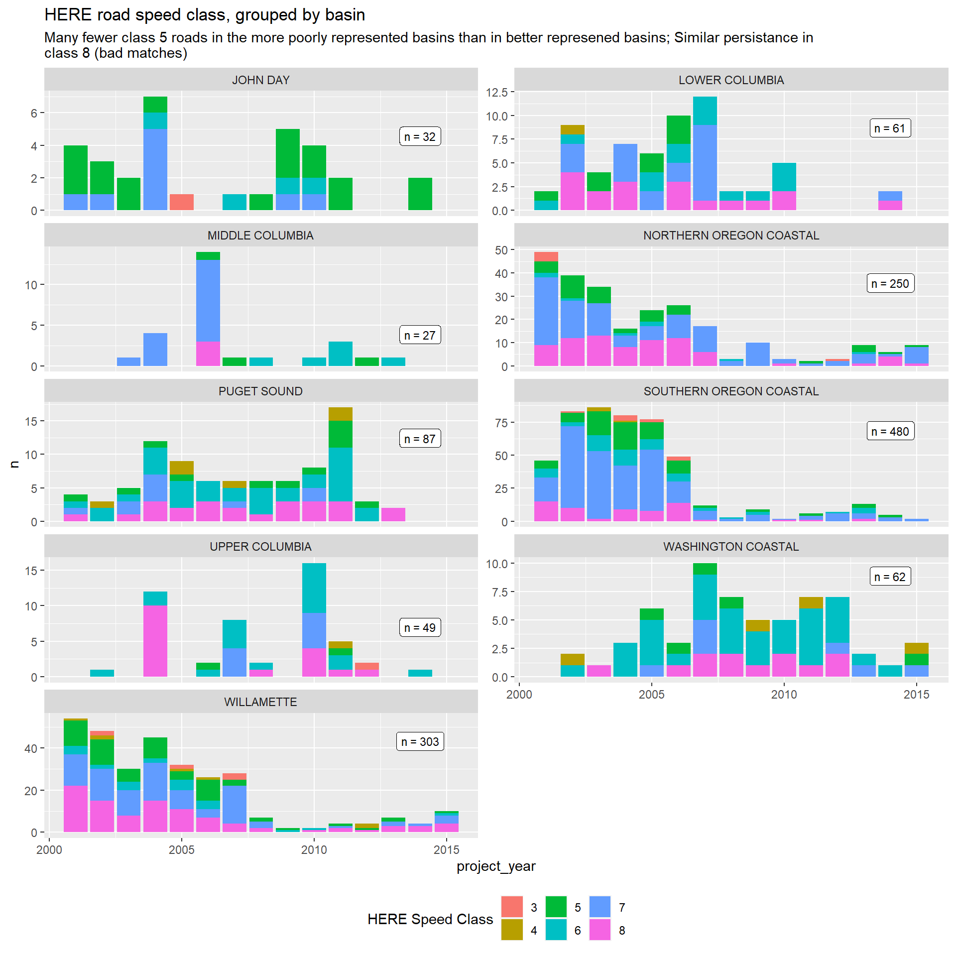
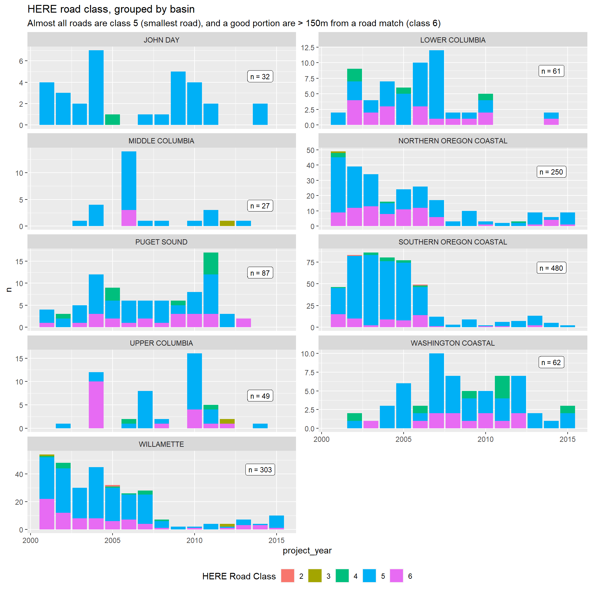
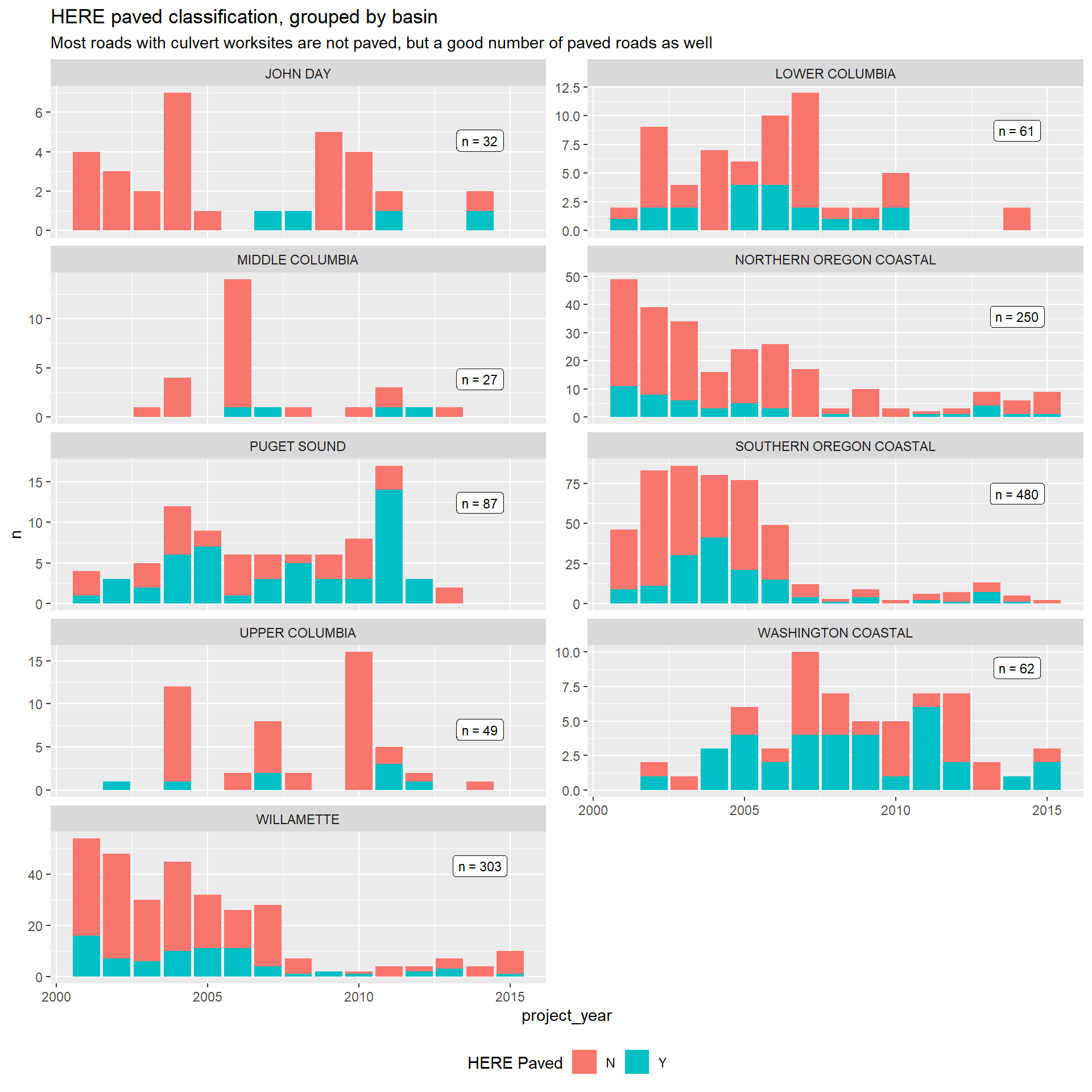
HERE roads: Speed, functional class, and paved
The HERE data provides variables for speed class, functional class, paved, and public. Paved status, speed class, and road type are potential cost drivers, indicating busier, larger roads that require longer fish crossings, more expensive construction on the affected road, and expected flagging costs associated with traffic diversion. Plots for all three are provided below.
| Classification | Value | Description |
|---|---|---|
| Functional class | 1 | Roads that allow for high volume, maximum speed traffic movement between and through major metropolitan areas. Functional class = 1 is applied to roads with very few, if any, speed changes. Access to the road is usually controlled. |
| 2 | Roads that are used to channel traffic to functional class = 1 roads for travel between and through cities in the shortest amount of time. Functional class = 2 is applied to roads with very few, if any speed changes that allow for high volume, high speed traffic movement. | |
| 3 | Roads which interconnect functional class = 2 roads and provide a high volume of traffic movement at a lower level of mobility than functional class = 2 roads. | |
| 4 | Roads which provide for a high volume of traffic movement at moderate speeds between neighbourhoods. These roads connect with higher functional class roads to collect and distribute traffic between neighbourhoods. | |
| 5 | Roads whose volume and traffic movement are below the level of any functional class. In addition, walkways, truck only roads, bus only roads, and emergency vehicle only roads receive functional class = 5. The following also receive functional class = 5: access roads, parking lanes, and connections internal to select pois in north america. Roads in marginal and illegal settlements in developing countries | |
| 6 | “Roads” associated with worksites > 150m from the nearest HERE road for here_class_badmatch. | |
| Speed category | 1 | > 130 kph / > 80 mph |
| 2 | 101-130 kph / 65-80 mph | |
| 3 | 91-100 kph / 55-64 mph | |
| 4 | 71-90 kph / 41-54 mph | |
| 5 | 51-70 kph / 31-40 mph | |
| 6 | 31-50 kph / 21-30 mph | |
| 7 | 11-30 kph / 6-20 mph | |
| 8 | < 11 kph / < 6 mph |
SalmonNet: Salmon habitat use
The StreamNet data provides variables for species and habitat use. These variables will be valuable for modeling benefits of culvert improvement, but may also lead to stricter design requirements if in the habitat of ESA listed species.
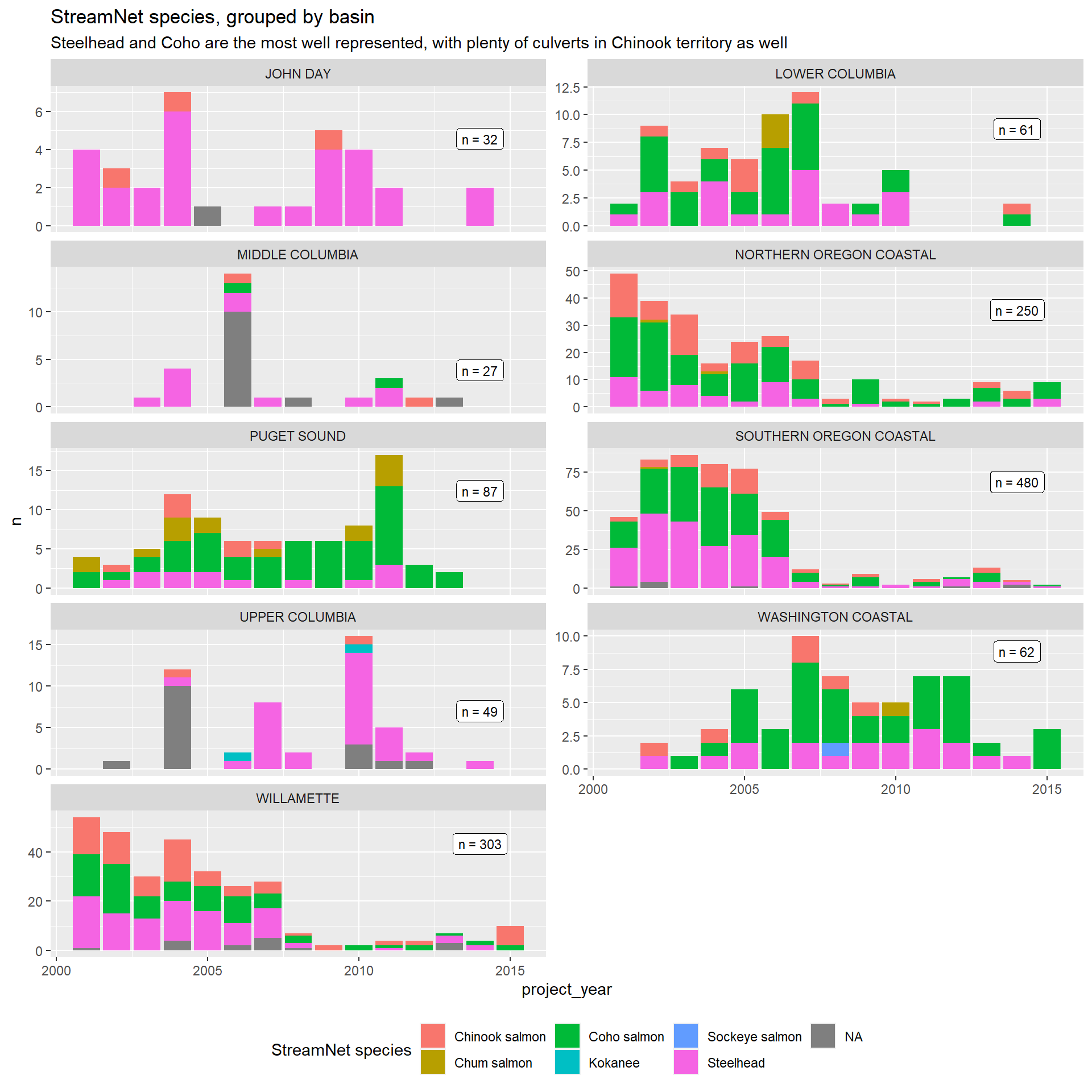
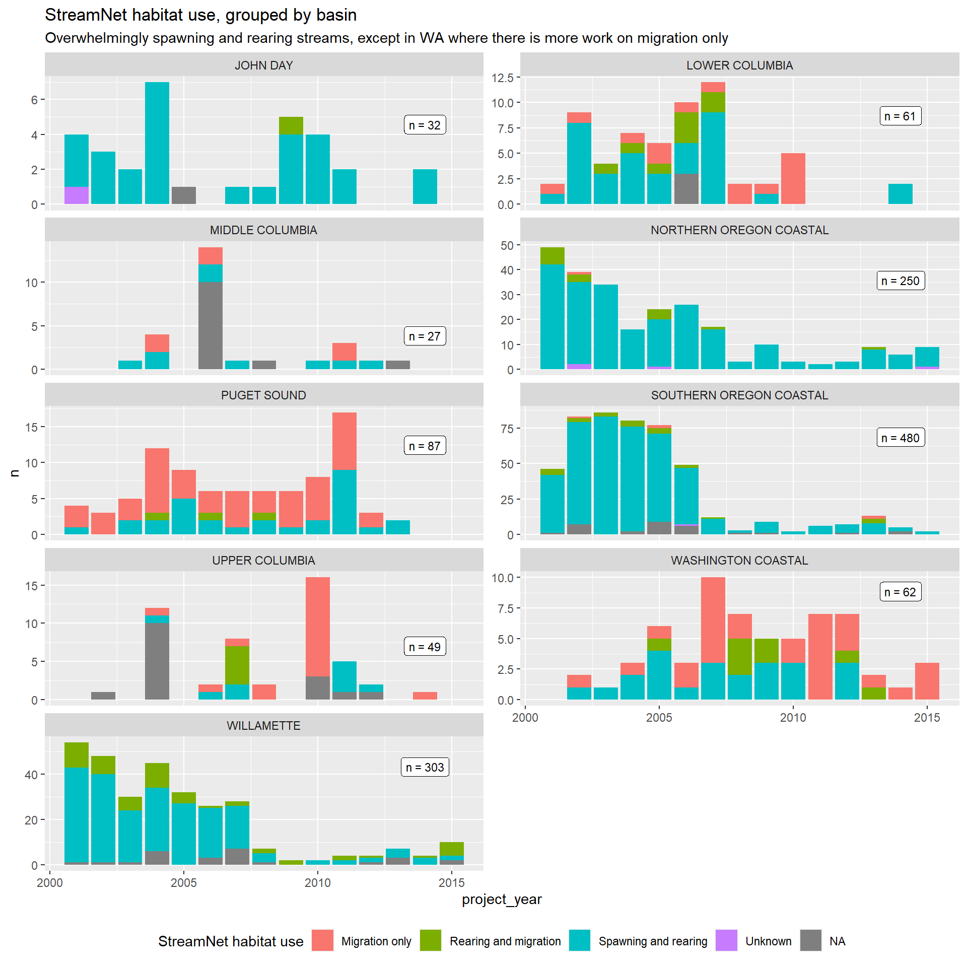
Key takeaway is that the culverts projects in Washington and Oregon are on distinctly different streams. In Washington, reported projects are more frequently on migration streams. These streams are likely to open up more upstream territory, but may also be wider and require more complex culvert designs. In Oregon, the reported projects are overwhelmingly on spawning and rearing streams, which (I believe) tend to be smaller and therefore would require less complex designs.
We can dig into attributes of associated NHDPlus streams and their associated catchments to further dig into this finding on the stream side.
NHDPlus attributes: Slope, bankfull width, and more
Stream characteristics are likely critical cost drivers. All state culvert design guidelines point to specific design needs for stream crossings when the crossing is either particularly wide (as measured by bankfull width) or at a steep slope (as measured by slope).
We gather these variables from NHDPlus Selected Attributes Version 2.1 (Wiezorek, Jackson, & Schwarz, 2018). by identifying the nearest NHDPlus stream object’s COMID and matching that COMID with the appropriate attributes. From the same database, we also gather population density, housing density, annual precipitation, road density, stream density, stream length, basin area, and NLCD land cover class share in the stream’s catchment.
These variables area also available aggregated over upstream networked NHDPlus streams and catchments, allowing for measures such as total upstream length and habitat features for associated catchments (e.g. road density, land cover, precipitation). These aggregated variables are calculated via two methods. Using the total method, all area in upstream catchments is weighted equally. Using the accumulated methods, area in upstream catchments is weighted by the proportion of flow that reaches the target catchment, accounting for natural and anthropogenic diversions.
For cost modeling, we focus on the bankfull width and slope variables. In the next steps, when benefit proxies are constructed for each culvert worksite, we can use the remaining variables to characterize upstream habitat with restored access.
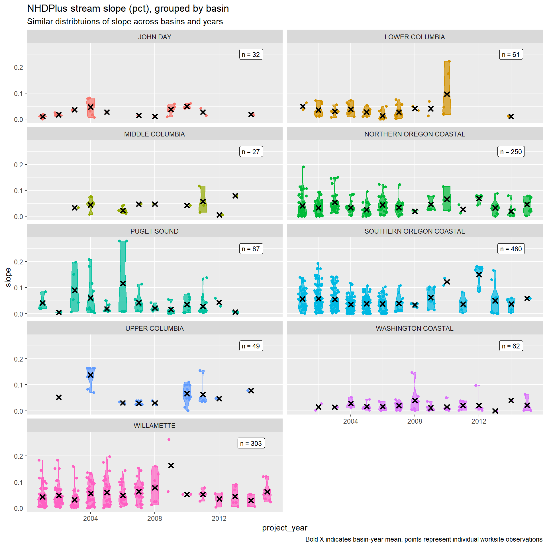
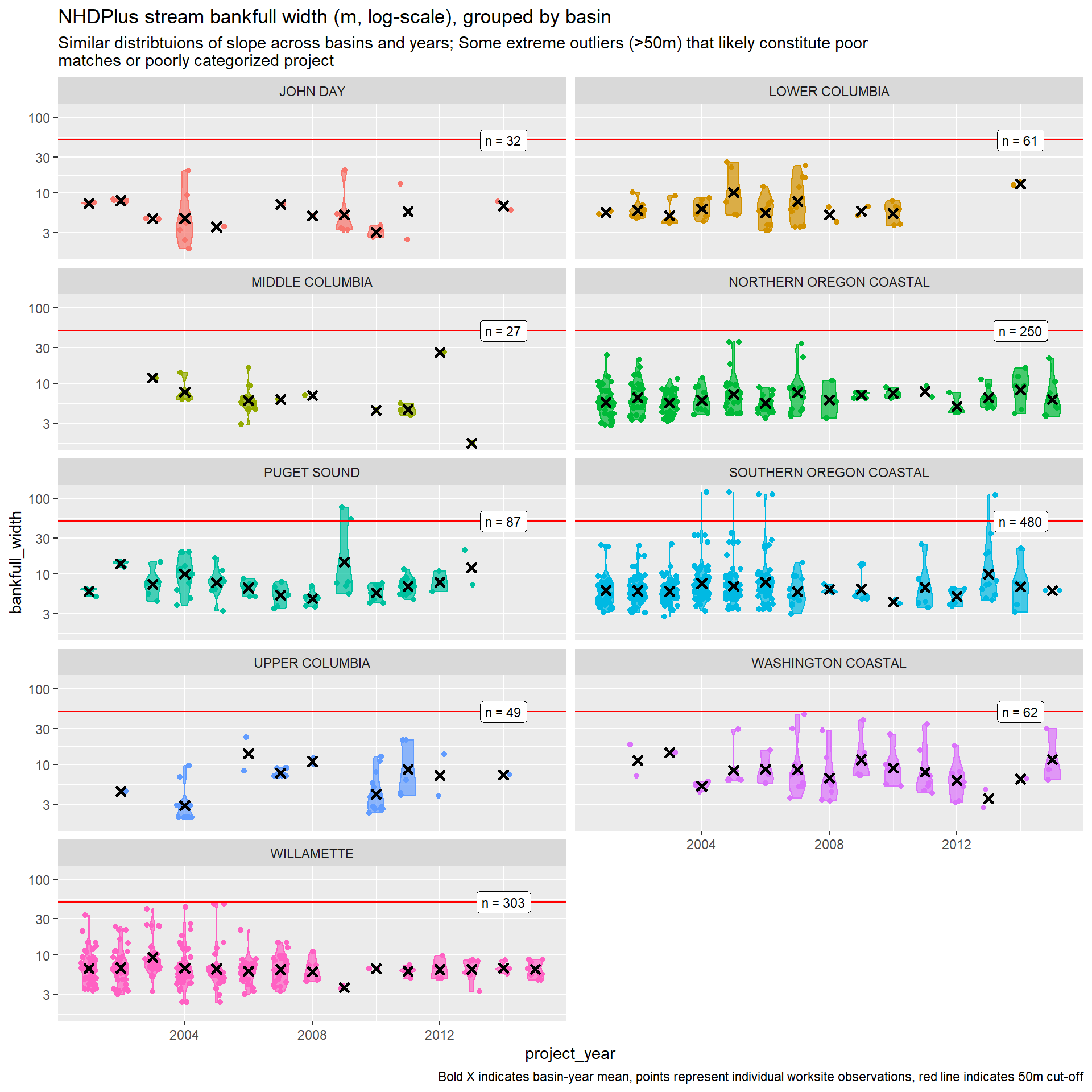
So it looks like the slope variable is pretty well behaved. We will drop worksites with bankfull width over 50m to remove extreme outliers.
sf_culv <-
  sf_culv %>%
  filter(
    bankfull_width < 50
  )
Otherwise, these variables show good behavior across these two physical attributes. Culverts in Washington are associated with larger streams, which will likely mean more expensive projects.
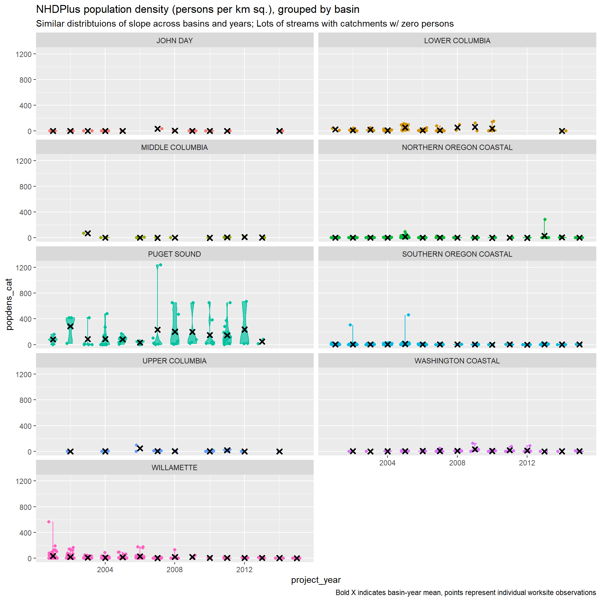
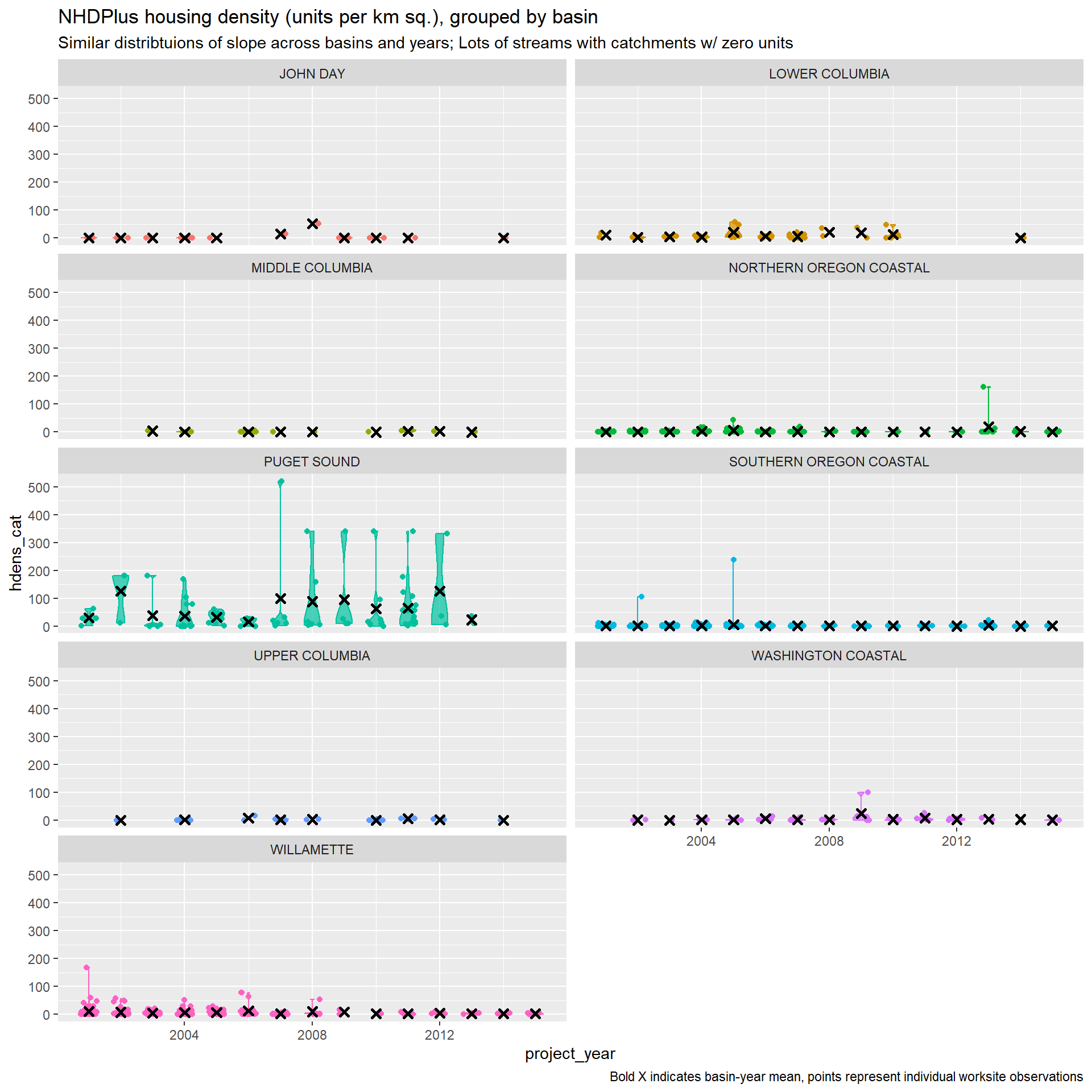
Population and housing density are highly correlated (Pearson’s coef. = 0.977), so we probably have to pick one or the other. Design documents point to site access as a crucial driver in project cost, and note that negotiating with private landowners can complicate projects. Housing density is a good proxy for this driver. Population density can be a good proxy for road traffic, which can increase flagging costs. Both effects are likely to increase costs. While we won’t be able to distinguish a mechanism, including either can control for density effects.
We should also consider alternative measures here that might better capture the hypothetical mechanisms at play. For example, variables such as the number of distinct parcels in the catchment, whether the worksite point is on public land, or the proportion of the catchment that is in public land might better capture increased costs due to access issues.
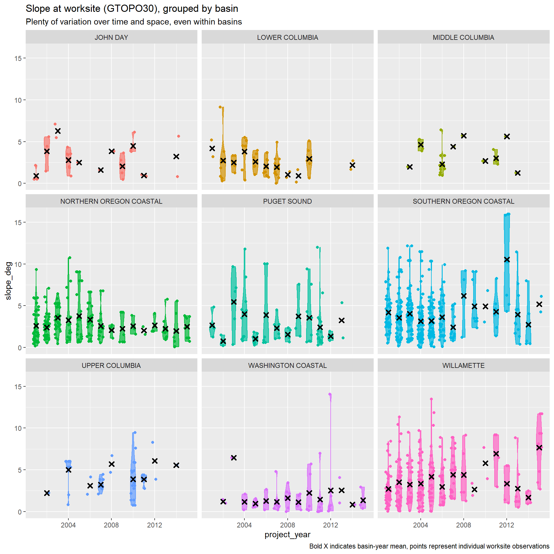
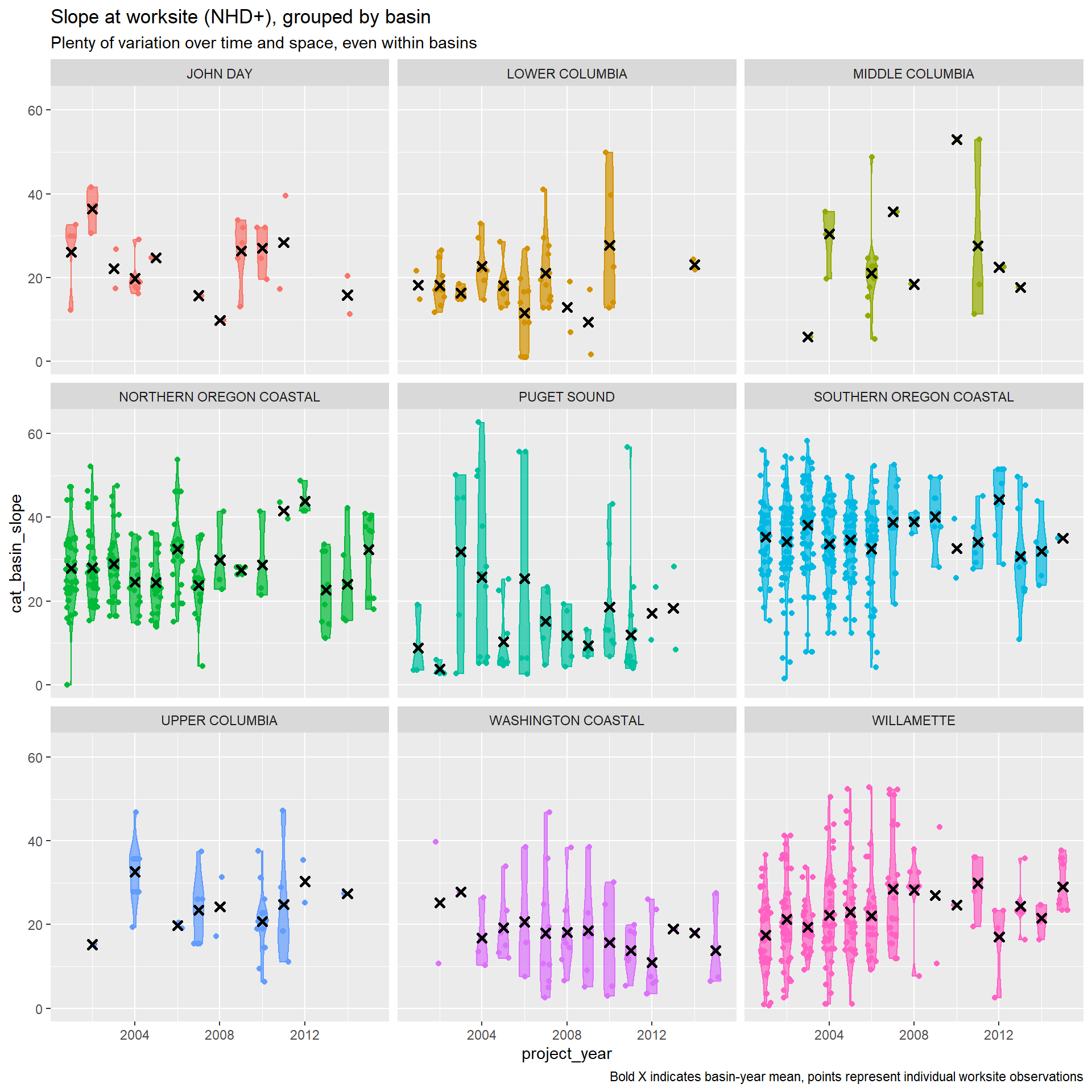
Slope at worksite
The slope at the worksite may increase project cost by restricting access to the culvert. We measure slope using the slope in degrees of the GTOPO30 grid cell the worksite falls in.
We can also measure slope using NHD+ attributes, which reports the slope of the catchment, distinct from the channel slope, for each stream segment.
Note that slope at worksites and the stream slope are distinct, both in their measurement and the mechanism through which they influence costs. Stream slope is our best available proxy for the slope of the stream at the culvert, which can require more complex, expensive culvert design to ensure fish passage. Slope at worksite is the land slope in the immediate vicinity of the culvert, which can restrict site access and available staging area, increasing project costs. While closely related, these are distinct (Pearson’s coef. = 0.533).
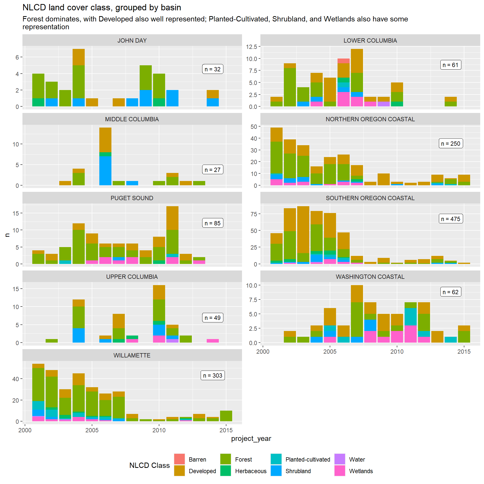
Land cover at worksites
Land cover can proxy for land use, which can effect how difficult it is to access and perform construction activities at the worksite, which may increase costs. It may also be correlated with road features (surface material, typical traffic, etc.) or stream features, and could be useful for providing more information for worksites where matches to roads and streams are poor.
The table below presents the NLCD land cover classifications. We use the “class” level of detail in the figures that follow.
| Class | Value | Classification | Description |
|---|---|---|---|
| Barren | 31 | Barren land (rock/sand/clay) | Areas of bedrock, desert pavement, scarps, talus, slides, volcanic material, glacial debris, sand dunes, strip mines, gravel pits and other accumulations of earthen material. Generally, vegetation accounts for less than 15% of total cover. |
| Developed | 21 | Developed, open space | Areas with a mixture of some constructed materials, but mostly vegetation in the form of lawn grasses. Impervious surfaces account for less than 20% of total cover. These areas most commonly include large-lot single-family housing units, parks, golf courses, and vegetation planted in developed settings for recreation, erosion control, or aesthetic purposes. |
| Developed | 22 | Developed, low intensity | Areas with a mixture of constructed materials and vegetation. Impervious surfaces account for 20% to 49% percent of total cover. These areas most commonly include single-family housing units. |
| Developed | 23 | Developed, medium intensity | Areas with a mixture of constructed materials and vegetation. Impervious surfaces account for 50% to 79% of the total cover. These areas most commonly include single-family housing units. |
| Developed | 24 | Developed high intensity | Highly developed areas where people reside or work in high numbers. Examples include apartment complexes, row houses and commercial/industrial. Impervious surfaces account for 80% to 100% of the total cover. |
| Forest | 41 | Deciduous forest | Areas dominated by trees generally greater than 5 meters tall, and greater than 20% of total vegetation cover. More than 75% of the tree species shed foliage simultaneously in response to seasonal change. |
| Forest | 42 | Evergreen forest | Areas dominated by trees generally greater than 5 meters tall, and greater than 20% of total vegetation cover. More than 75% of the tree species maintain their leaves all year. Canopy is never without green foliage. |
| Forest | 43 | Mixed forest | Areas dominated by trees generally greater than 5 meters tall, and greater than 20% of total vegetation cover. Neither deciduous nor evergreen species are greater than 75% of total tree cover. |
| Herbaceous | 71 | Grassland/herbaceous | Areas dominated by gramanoid or herbaceous vegetation, generally greater than 80% of total vegetation. These areas are not subject to intensive management such as tilling, but can be utilized for grazing. |
| Planted-cultivated | 81 | Pasture/hay-areas of grasses, legumes, or grass | Legume mixtures planted for livestock grazing or the production of seed or hay crops, typically on a perennial cycle. Pasture/hay vegetation accounts for greater than 20% of total vegetation. |
| Planted-cultivated | 82 | Cultivated crops | Areas used for the production of annual crops, such as corn, soybeans, vegetables, tobacco, and cotton, and also perennial woody crops such as orchards and vineyards. Crop vegetation accounts for greater than 20% of total vegetation. This class also includes all land being actively tilled. |
| Shrubland | 52 | Shrub/scrub | Areas dominated by shrubs; less than 5 meters tall with shrub canopy typically greater than 20% of total vegetation. This class includes true shrubs, young trees in an early successional stage or trees stunted from environmental conditions. |
| Water | 11 | Open water | Areas of open water, generally with less than 25% cover of vegetation or soil. |
| Water | 12 | Perennial ice/snow | Areas characterized by a perennial cover of ice and/or snow, generally greater than 25% of total cover. |
| Wetlands | 90 | Woody wetlands | Areas where forest or shrubland vegetation accounts for greater than 20% of vegetative cover and the soil or substrate is periodically saturated with or covered with water. |
| Wetlands | 95 | Emergent herbaceous wetlands | Areas where perennial herbaceous vegetation accounts for greater than 80% of vegetative cover and the soil or substrate is periodically saturated with or covered with water. |
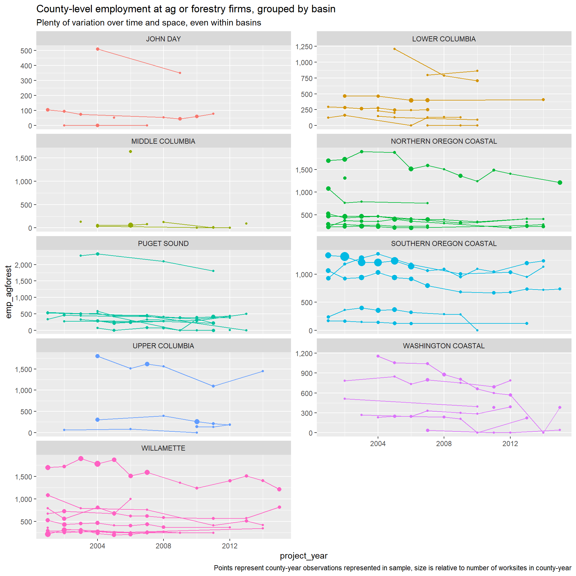
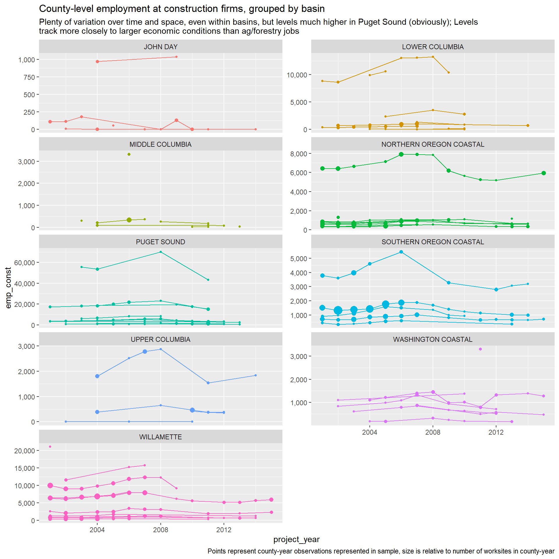
Job shares in relevant sectors
To capture labor market patterns that might affect culvert costs, we collect the number of jobs for construction and ag/forestry NAICS codes for the county the worksite is located in via County Business Patterns. Access to experienced labor can keep costs down. These variables are intended to capture that effect.
Because counties are so large in Oregon and Washington, this is not the ideal measure of job patterns. For example, culverts in rural King County will have jobs numbers driven largely by patterns in Seattle, despite being as much as 40 miles away. Other ideas on how to capture these effects would be appreciated!
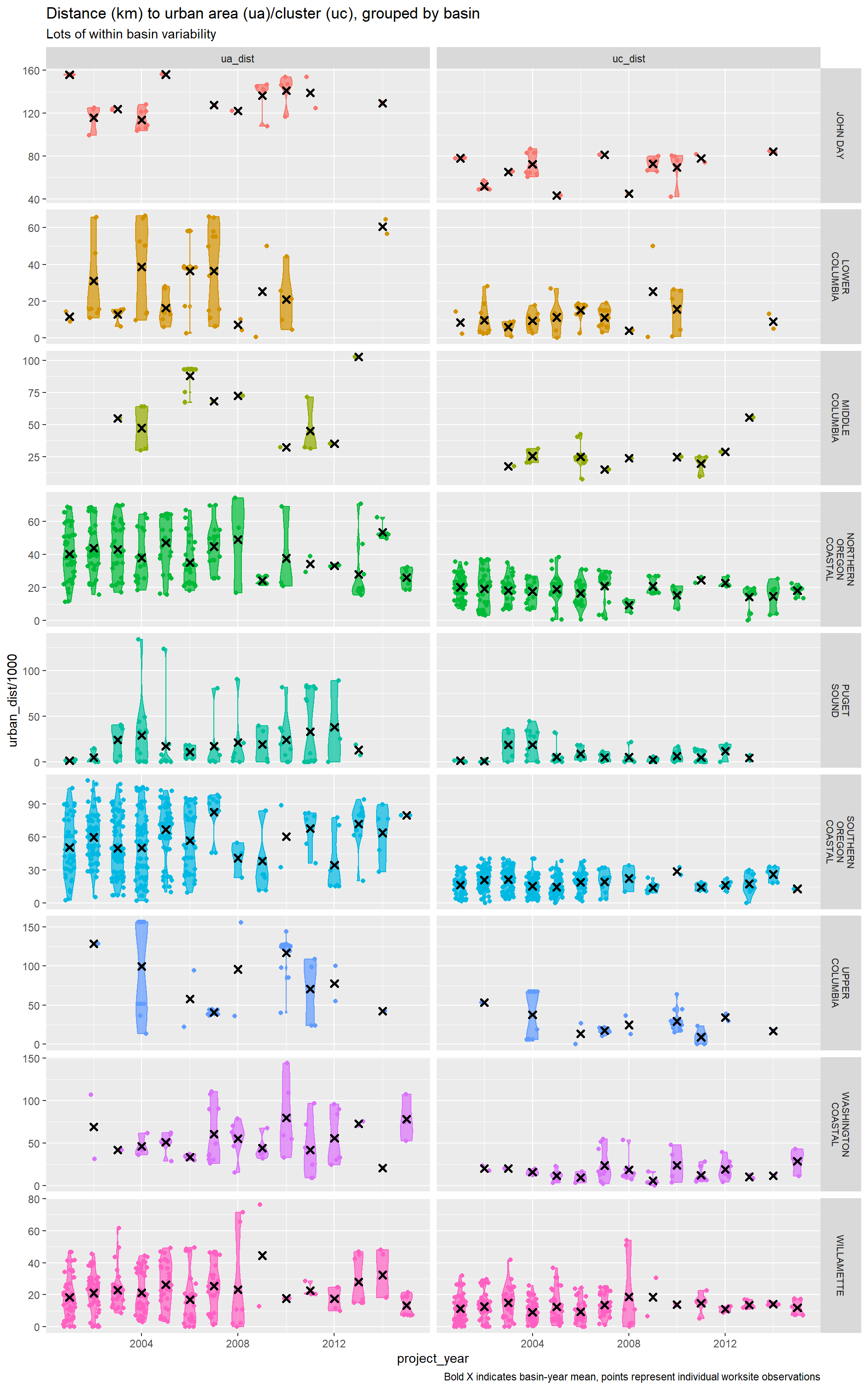
US Census: Distance to population center
We proxy for availability of supplies and labor by measuring the distance from each worksite to the boundary of census designated “Urban Areas” and “Urban Clusters” as of the 2010 census (source). Urban areas are defined as contiguous areas of 50,000 or more people, while urban clusters are defined as contiguous areas of 2,500 to 50,000 people. (Worksites within urban areas/clusters are assigned 0.)
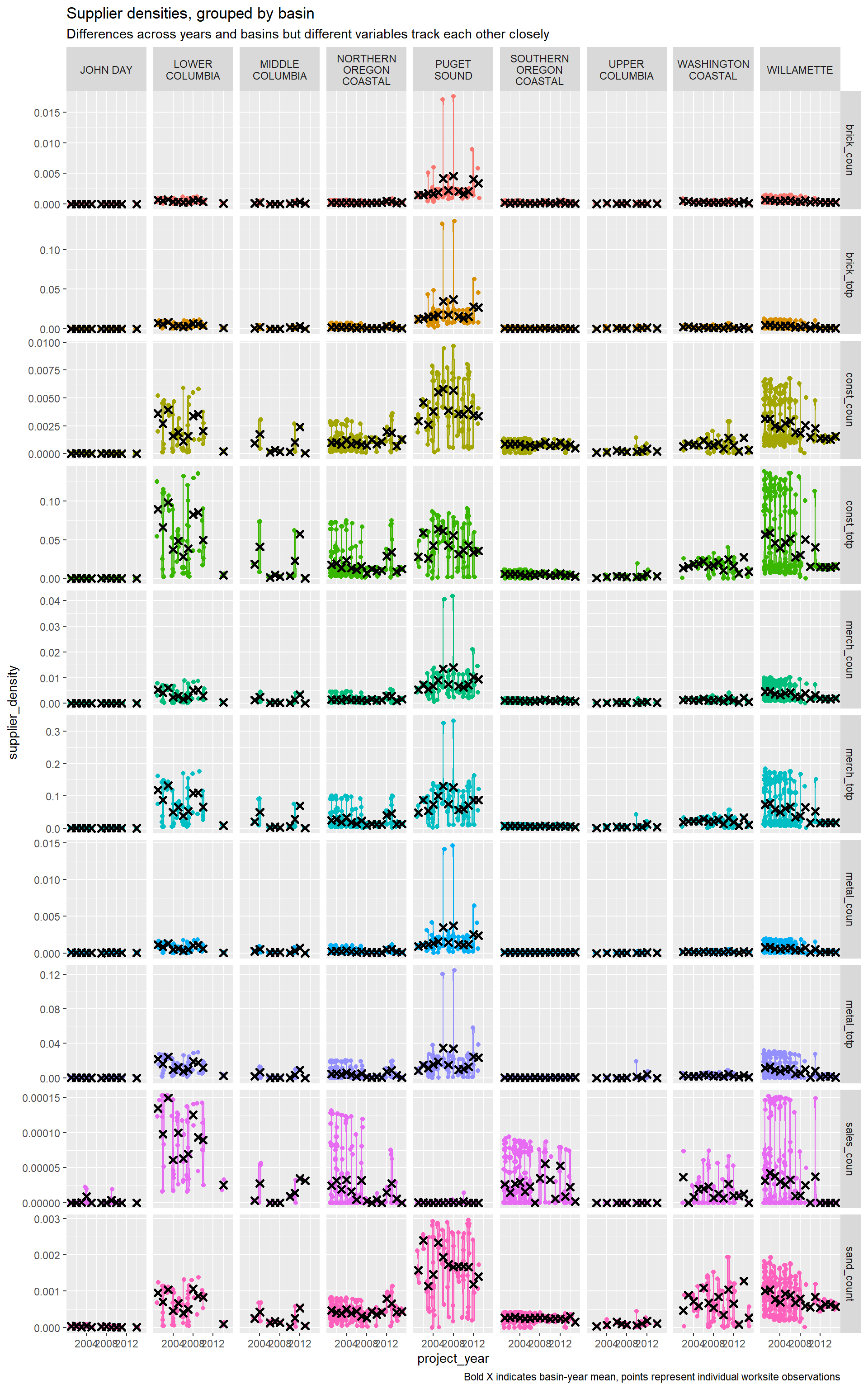
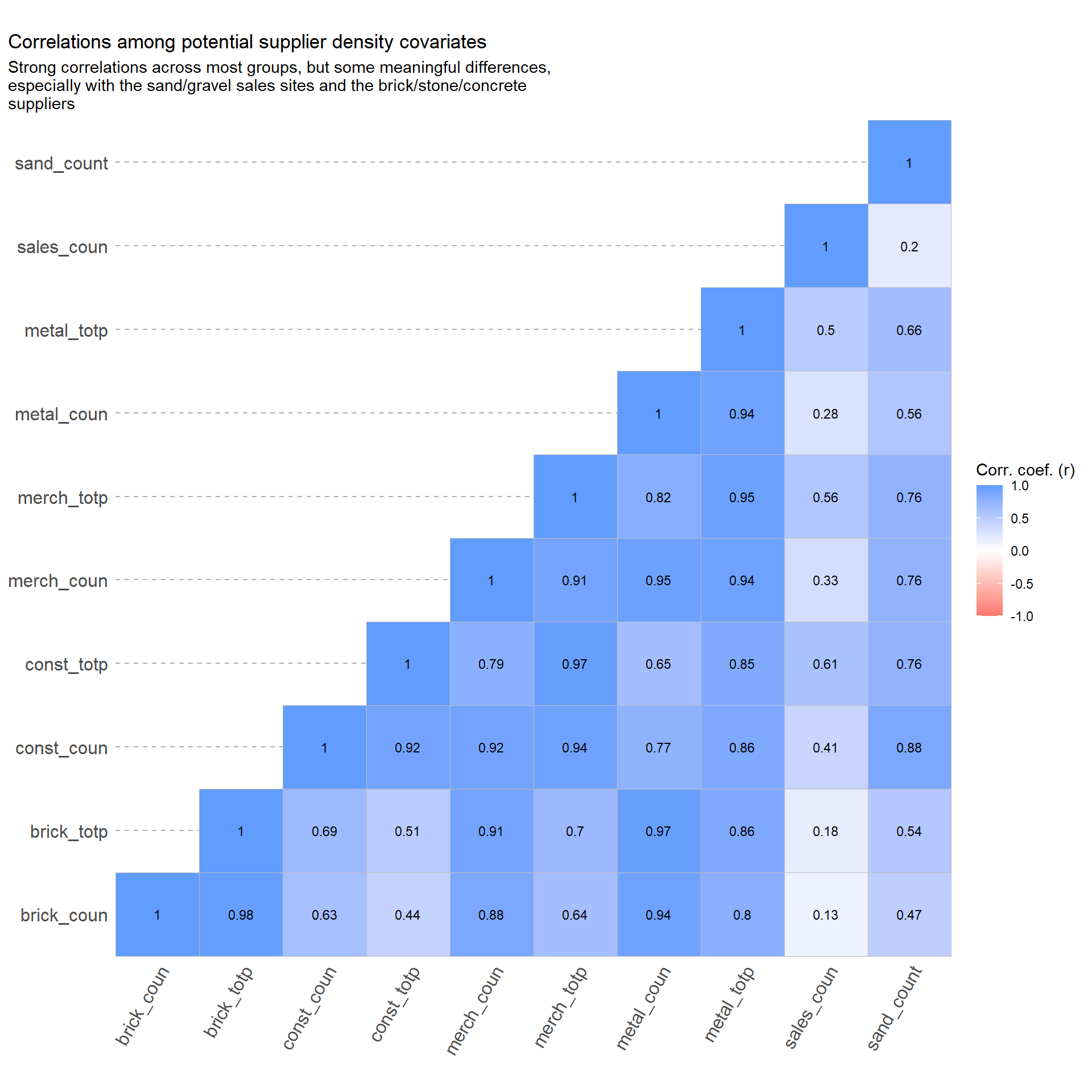
HIFLD: Material supply operation density
We proxy for availability of raw materials and machinery by generating a kernel density field for operations identified in the following NAICS categories:
- Merchant Wholesalers Durable Goods: Brick, Stone and Related (brick_coun/brick_totp)
- Merchant Wholesalers Durable Goods: Construction and Mining (const_coun/counst_top)
- Merchant Wholesalers Durable Goods: Metals Service Centers (metal_coun/metal_top)
- Merchant Wholesalers Durable Goods: All above sub-categores (merch_coun/merch_top)
- Sand & Gravel Operations: Sales Yard (sales_coun)
- Sand & Gravel Operations: All sub-categories, incl. Sales Yard (sand_count)
For the “Merchant Wholesalers Durable Goods” categories we include densities based on both simple site count (*_coun) and weighted by persons/site to scale for operation size (*_totp). For Sand & Graveel Operations, only simple site count densities are estimated as persons/site data is unavailable.
BLM: Surface jurisdiction of land
We are also interested in public land and private land nearby worksites as a proxy for land access. We identify the proportion of land ownership by group within 500m, 1km, and 2.5km radius circular buffer of each worksite using BLM surface jurisdiction records from 2019. (Blake could you provide more detailed sourcing on these data?). We distinguish between the following ownership entities:
key_blm <- read_xlsx(here("data/Culverts spatial overlays v 20Jan2021.xlsx"), sheet = 5) %>%
  as_tibble() %>%
  filter(Present == 1) %>%
  mutate(Present = NULL)

key_blm %>%
  arrange(Code) %>%
  kable(caption = "Value key for BLM land ownership variables") %>%
  kable_styling() %>%
  collapse_rows(
    1,
    valign = "top",
    row_group_label_position = "stacked",
    headers_to_remove = 1
)| Code | Description |
|---|---|
| BIA | Bureau of Indian Affairs |
| BLM | Bureau of Land Management |
| BPA | Bonneville Power Administration |
| COE | Corps of Engineers |
| FWS | U.S. Fish and Wildlife Service |
| GSA | General Services Administration |
| LG | Local Government |
| NPS | National Park Service |
| PV | Private Individual or Company |
| PVI | Lands Managed by Private Industry |
| PVN | Private Non-Industrial Owner |
| PVU | Private Urban Lands |
| ST | State Agency |
| STF | State Dept. of Forestry |
| STL | Division of State Lands |
| STP | State Dept. of Parks and Recreation |
| STW | State Dept. of Fish and Wildlife |
| UND | Undetermined |
| USFS | U.S. Forest Service |
| WATER | Water |
Lands managed by private industry in this context refer mainly to forestry activities. High values indicate that the culvert in question is likely owned by a timber company replacing the barrier under state forestland policies.
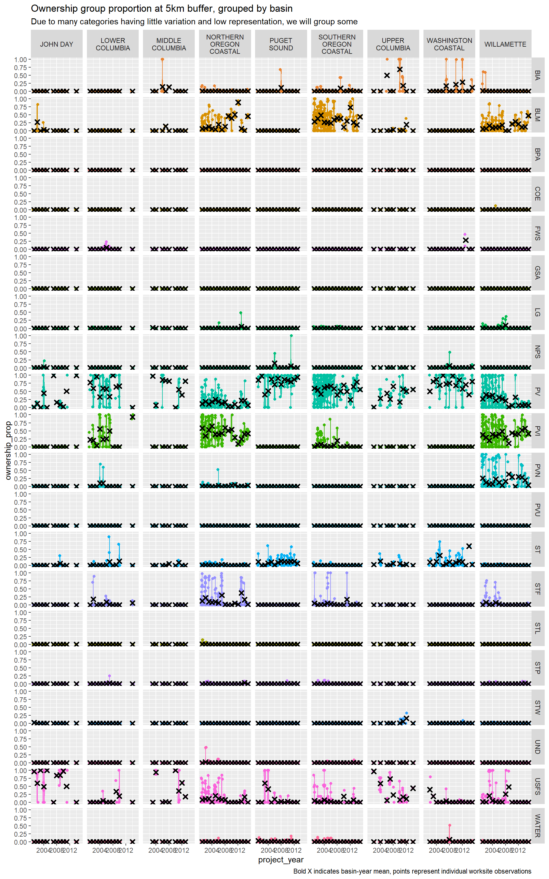
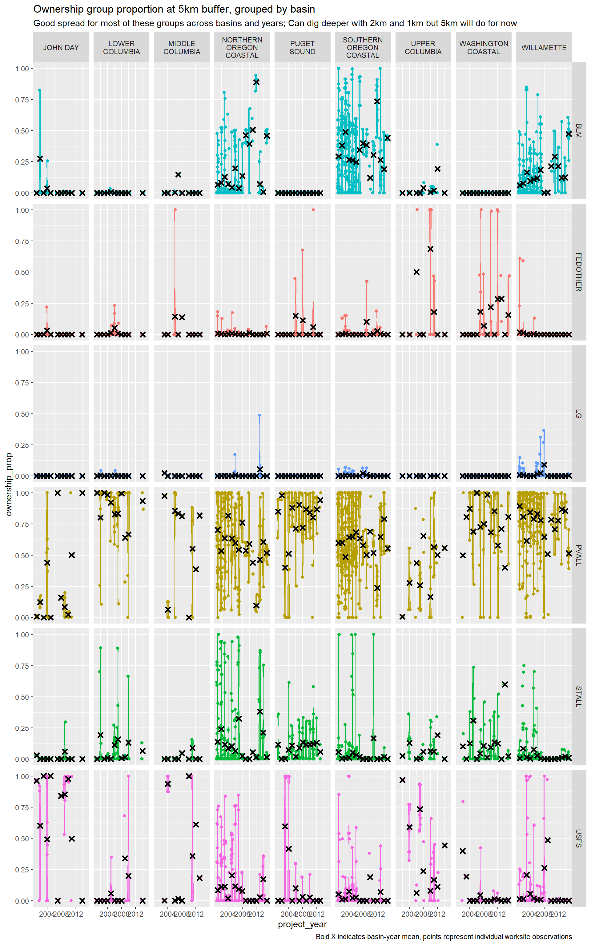
We also provide summaries for composite variables that group private land, state-managed land, and federally-managed land (other than BLM and USFS, which manage significant amounts on their onw) by summing across relevant variables.
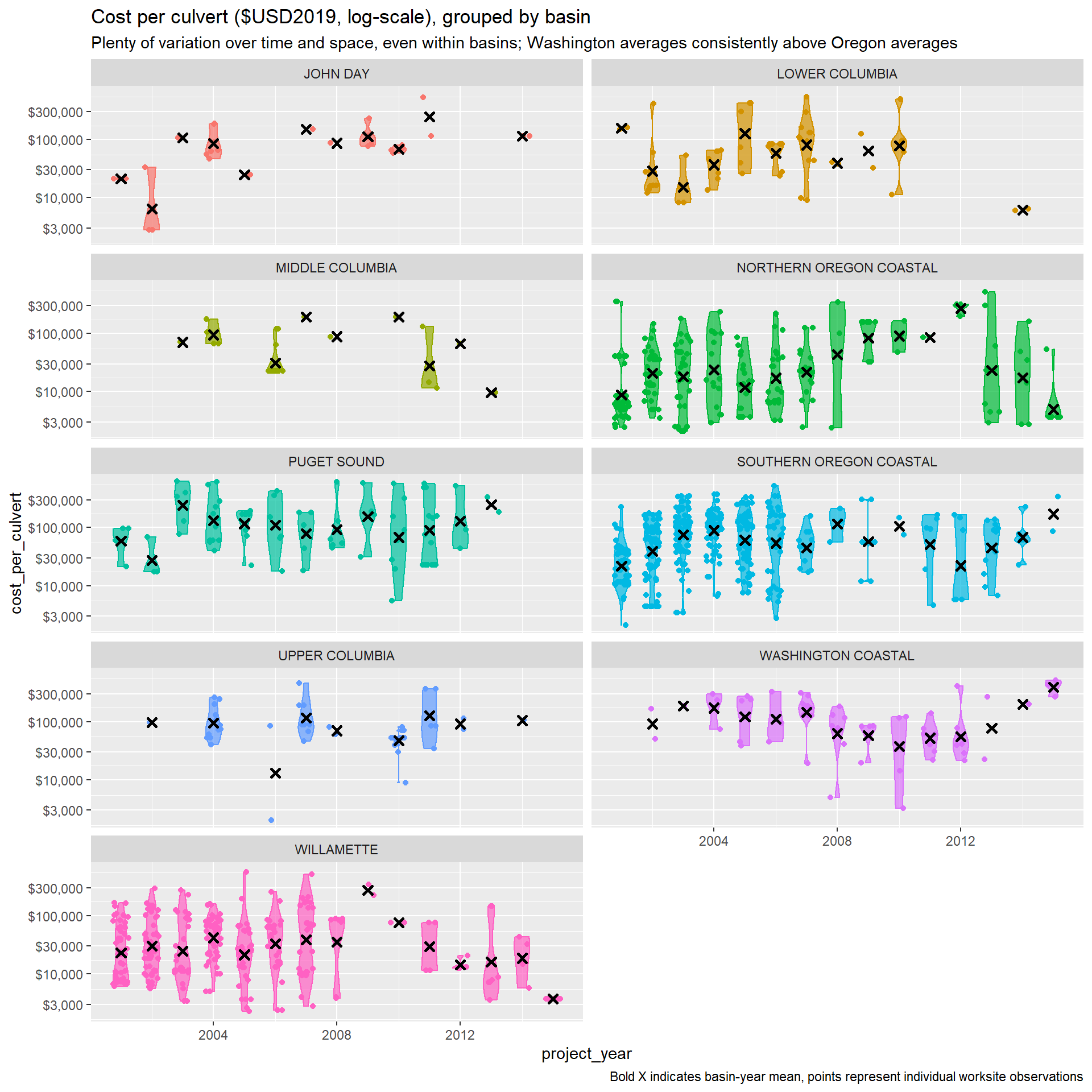
PNSHP: Culvert project costs
Culvert project costs are the primary dependent variable in this study. We calculate cost per culvert at the project level by first tallying the number of culverts installed, upgraded, or removed at the project level. We then divide project-level costs by the number of culverts. This cost per culvert measure is assigned to each worksite associated with that project.
Key takeaways
There are noticeable differences between Washington and Oregon culvert projects represented in the data. Washington projects tend to more frequently be on migration routes and on paved roads, and on wider streams. Oregon projects are more likely to be on spawning and rearing streams, unpaved roads, and on narrower streams. This likely goes a long way in explaining the large differences in costs across the two states, but can be accounted for with thoughtful inclusion of covariates in the conditioning set.
The PNSHP culverts data also over-represent smaller, unpaved roads across the board. This limits the usefulness of the data for projecting costs for passage improvements on larger roads (i.e., with speed limits >40 mph). These limitations are likely to be reflected by larger standard errors on any estimates of marginal effects, but should be noted with any presentation of results.
Finally, a version of the proceeding analysis of the potential explanatory variables will be conducted for the fish passage barrier inventories maintained by Oregon and Washington Departments of Fish and Wildlife. This exercise will reveal how representative the PNSHP projects are relative to potential future projects.
# Render output
# rmarkdown::render(here::here("R/C.culvertsspatial/06.spatialexplore.R"), output_file = here::here("output/culvertsspatial_report_2020sep24.html"))
sessionInfo()R version 4.0.2 (2020-06-22)
Platform: x86_64-w64-mingw32/x64 (64-bit)
Running under: Windows 10 x64 (build 19041)
Matrix products: default
locale:
[1] LC_COLLATE=English_United States.1252
[2] LC_CTYPE=English_United States.1252
[3] LC_MONETARY=English_United States.1252
[4] LC_NUMERIC=C
[5] LC_TIME=English_United States.1252
attached base packages:
[1] stats graphics grDevices utils datasets methods base
other attached packages:
[1] mctest_1.3.1 ggcorrplot_0.1.3 kableExtra_1.1.0 knitr_1.29
[5] rmarkdown_2.3 janitor_2.0.1 readxl_1.3.1 sf_0.9-5
[9] here_0.1 forcats_0.5.0 stringr_1.4.0 dplyr_1.0.1
[13] purrr_0.3.4 readr_1.3.1 tidyr_1.1.1 tibble_3.0.4
[17] ggplot2_3.3.2 tidyverse_1.3.0 scales_1.1.1 workflowr_1.6.2
loaded via a namespace (and not attached):
[1] httr_1.4.2 jsonlite_1.7.1 viridisLite_0.3.0 modelr_0.1.8
[5] assertthat_0.2.1 highr_0.8 selectr_0.4-2 blob_1.2.1
[9] cellranger_1.1.0 yaml_2.2.1 pillar_1.4.6 backports_1.1.8
[13] glue_1.4.2 digest_0.6.25 promises_1.1.1 rvest_0.3.6
[17] snakecase_0.11.0 colorspace_1.4-1 plyr_1.8.6 htmltools_0.5.0
[21] httpuv_1.5.4 pkgconfig_2.0.3 broom_0.7.0 haven_2.3.1
[25] webshot_0.5.2 later_1.1.0.1 git2r_0.27.1 generics_0.0.2
[29] farver_2.0.3 ellipsis_0.3.1 withr_2.2.0 cli_2.1.0
[33] magrittr_1.5 crayon_1.3.4 evaluate_0.14 ps_1.3.3
[37] fs_1.4.2 fansi_0.4.1 xml2_1.3.2 class_7.3-17
[41] tools_4.0.2 hms_0.5.3 lifecycle_0.2.0 munsell_0.5.0
[45] reprex_0.3.0 compiler_4.0.2 e1071_1.7-3 rlang_0.4.8
[49] classInt_0.4-3 units_0.6-7 grid_4.0.2 rstudioapi_0.11
[53] labeling_0.3 gtable_0.3.0 DBI_1.1.0 reshape2_1.4.4
[57] R6_2.4.1 lubridate_1.7.9 utf8_1.1.4 rprojroot_1.3-2
[61] KernSmooth_2.23-17 stringi_1.4.6 Rcpp_1.0.5 vctrs_0.3.4
[65] dbplyr_1.4.4 tidyselect_1.1.0 xfun_0.16